


Contents
Scroll to:
https://doi.org/10.5800/GT-2024-15-4-0777
EDN: ELARBH
Scroll to:
Dynamic rupture scenarios on various fault geometries are studied extensively in the literature for domains with the planar top surface. However, landscapes on the earth, particularly in tectonic regimes, can undulate upwards or downwards depending on faulting conditions. In this paper, we studied a dipping fault model with a dip fault angle of 60 degrees, inspired by the 2D version of dynamic rupture benchmark TPV10 from the Southern California Earthquake Center (SCEC). A topographic feature adjacent to the fault is introduced in the form of a hill or a valley. The shape of the undulation was varied from semi-circular form to Gaussian profile. This paper examines the impact of topographic features (valleys or hills) on slip amplitude on a fault. The distance at which the features exist also affects the amount of slip on fault, ruptured in that region. The results for a couple of different radii of semi-circular formation and equivalent standard deviation of Gaussian undulation are also summarized in this paper. The study depicts that the topography in the vicinity of the fault can affect the magnitude of slip propagation on fault surface.
Parla R., Somala S.N. INFLUENCE OF HILLS AND VALLEYS ON FREE SURFACE SLIP AMPLIFICATION IN DYNAMIC RUPTURE ON A DIPPING FAULT. Geodynamics & Tectonophysics. 2024;15(4):0777. https://doi.org/10.5800/GT-2024-15-4-0777. EDN: ELARBH
Slip at the intersection of a fault with a free surface determines the amount of distance by which a structure across the fault gets torn apart and is separated from the portions on each side. Higher slip leads to a larger offset and in case of dipping faults can introduce both vertical and horizontal offsets. The past studies exploring the effect of free surface on rupture dynamics were confined to flat terrain for simplifying the numerical simulations [Chen, Zhang, 2006; Zhang, Chen, 2006a, 2006b; Day et al., 2008; Kaneko, Lapusta, 2010; Xu et al., 2015]. However, the undulations of the earth’s surface differ from one place to another and exhibit an irregular pattern of topography. [Ely et al., 2010] demonstrated that the surface topography has a significant effect on rupture dynamics by modelling the southern San Andrea Fault rupture. [Zhang et al., 2016] exclusively studied the effect of topography on rupture propagation and sub-shear to super-shear transition by comparing rupture dynamics on faults with different topographic features in their models. [Huang et al., 2018] investigated the effect of canyon-shaped and hill-shaped topography on near-fault ground motion using curved-grid-finite-difference models (CGFDM) and concluded that the canyon-shaped topography has a stronger effect on near-fault ground motion compared to the hill-shaped topography. Understanding whether the presence of such topographic features as hills or valleys in case of faults reaching the free surface is a boon or curse would be useful since the construction of any structure across the fault boundary is inevitable due to either lack of land elsewhere or habitat resource availability. Our preliminary results depict that topography in the vicinity of the fault can change the magnitude of slip along the fault. Fences along some bordering countries could also be found among these structures but the damage to a fence may not necessarily have a profound impact on the economy of any country.
Earthquake modelling can range from a simple double couple point source to spontaneous rupture propagation on finite faults governed by frictional contact laws. Many researchers in the past years adopted numerous numerical and analytical methods to solve both point source and spontaneous rupture problems [Zhang, Chen, 2006a, 2006b; Andrews, 1976; Madariaga, 1976; Das, Aki, 1977; Fukuyama, Madariaga, 1998; Aochi et al., 2000; Oglesby et al., 2000a, 2000b; Day et al., 2005; Benjemaa et al., 2007, 2009; Kaneko et al., 2008; Ely et al., 2009; Hok, Fukuyama, 2011; Tago et al., 2012; Zhang et al., 2014; Parla, Somala, 2022a, 2022b; Parla et al., 2022; Somala et al., 2022]. While an earthquake modelled as a spontaneous rupture is dependent on the initial conditions which are often insufficiently known, the spontaneous rupture propagation popularly termed as a dynamic rupture is by far the best possible way of modelling an earthquake. [Hok, Fukuyama, 2011] have modelled the dynamic rupture propagation on shallow dipping fault using the boundary integral equation method (BIEM) to study the effect of free surface on rupture characteristics by introducing virtual free-surface elements. Kinematic ruptures, based on a statistical relation for fault slip obtained from kinematic inversions of earthquake data, will just give as much slip as we prescribe at the junction of a topographic feature and a fault, and are thus considered as if they were not used to understand differences in a slip near the free surface due to topographic feature, while keeping all other conditions the same.
The Southern California Earthquake Center (SCEC) has put together several benchmarks for validation of numerical implementations of dynamic rupture by the researchers [Harris et al., 2009]. Dynamic rupture simulations in this paper are performed using PyLith [Aagaard et al., 2013], a code that is benchmarked with the SCEC dynamic rupture benchmarks. This study addresses the free surface slip amplification owing to the influence of topographic features of a certain class by choosing a TPV10 benchmark from the SCEC dynamic rupture benchmarks. In this study, we constrain ourselves to 2D cases.
PyLith, the software chosen to run dynamic rupture simulations in this study, is based on the finite element method of converting strong form of elasto-dynamic equation to weak. For brevity, we outline the solution method for quasi-static problems using only index notation. In quasi-static problems, with neglect of the inertial terms, the reduced weak form of equation will be:

We solve this equation through formulation of a linear algebraic system of equations (Au=b), involving the residual (r=b–Au) and Jacobian (A). The residual is simply:


Combining the expressions for the increment in stresses and making use of the symmetry of the weighting functions, the Jacobian matrix will be:

where σij – stress tensor field, V – volume bounded by surface S, Ti – traction vector field, u – displacement, t – time.
The detailed solution method for quasi-static problem can be referred to PyLith manual [Aagaard et al., 2010] (section 2.3). The domain is discretized into triangular elements and the field variable (displacement in this case) is considered to be varying linearly within the element. Integrals are used as approximation to summation over all the elements and summation over function values evaluated at Gauss quadrature points multiplied by corresponding weights and the Jacobian. The weak form so obtained is solved by minimizing the residual in an iterative fashion after discretizing in time using Newmark’s explicit time-stepping scheme [Aagaard et al., 2010]. While this gives the equations for the bulk domain in terms of displacement, the contact friction conditions are imposed on the fault such that friction is governed by slip-weakening law and interpenetration is avoided. The fault is replaced by zero volume cohesive elements which have additional degrees of freedom in terms of Lagrange multipliers [Aagaard et al., 2010]. These Lagrange multipliers are the energy conjugate of displacements, the tractions. Excess shear tractions over and above the frictional strength get converted into the slip in the direction of resultant shear traction. This constraint is solved together with the weak form discretized in time to obtain displacement field and the spatiotemporal evolution of slip on the fault.
The material properties of the model and the initial traction parameters on fault are taken as per 2D version of TPV10 SCEC (Southern California Earthquake Centre) benchmark model. The 2D version of TPV10 SCEC dynamic rupture benchmark [Harris et al., 2009], taken as the reference point, is shown in Fig. 1. The domain is a uniform half-space, and the medium is characterized by the P-wave velocity of 5.72 km/s and S-wave velocity of 3.3 km/s. Mass per unit volume of the material in the medium is 2.7 g/cc. The 2D fault reveals a mechanism of thrust fault rupture with 60° dip and 90° rake angles, reaching the free surface with a length of 15 km. Plane strain assumption is used with a vertical cross-section of the TPV10 benchmark to solve its 2D version. The rupture process on fault is governed by slip-weakening friction law [Ida, 1972]. The linear slip-weakening friction model produces shear tractions equal to the cohesive stress plus a contribution proportional to the fault normal traction that decreases from static to dynamic value as slip progresses. The friction stress on fault will follow the equation:
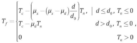
where µs is static coefficient of friction, µd is dynamic coefficient of friction, d0 is slip weakening parameter, d is cumulative slip, Tc is cohesive stress, Tn is normal stress, and Tf is shear traction on fault.
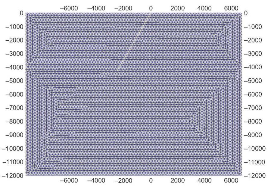
Fig. 1. Geometry of reference case. White line denotes the fault.
Рис. 1. Геометрия эталонной модели. Белой линией обозначен разлом.
Nucleation is carried out on a 3 km patch located at 12 km down-dip having static and dynamic friction coefficients of 0.76 and 0.448, respectively, and a critical slip-weakening distance of 0.5 m.
Cohesion on the fault is chosen to be 0.2 MPa. Meshing is done with 200m triangular elements. Failure follows the linear slip-weakening law [Ida, 1972]. Initial tractions are assumed to follow a depth-dependent behavior where normal traction increases as 7378 Pa/m along with down-dip distance and the ratio of shear traction to normal traction is 0.55 except on a 3 km nucleation where the shear traction is 67.99 MPa. Shear traction exceeds frictional strength only on the nucleation path where rupture starts and propagates spontaneously.
To understand the free surface slip amplification due to a pure upward undulation (hill) and a pure downward undulation (valley) near the fault, we first consider four cases as shown in Fig. 2. The shape of a valley as well as that of a hill is taken as a 1 km radius semi-circle at first and then as a 2 km radius semi-circle. The topographic features considered in this study (including hill and valley) are having dimension as shown in Table 1. The final slip as a function of horizontal distance for these four cases is also plotted in Fig. 3, along with the final slip for the reference case. It can be seen from Fig. 3 that the slip is amplified by a valley like a feature near the intersection of a free surface with the fault. More slip is observed with an increase in the semi-circular valley feature. For a 1 km radius semi-circular valley, peak slip is still at the nucleation patch similar to the reference configuration. However, in case of a 2 km radius semi-circular valley, peak slip occurs near the free surface and is almost twice that of the reference configuration. This could be due to the narrow corner formed near the intersection of a free surface with the fault and a potentially greater surface area of the semi-circular feature on the path taken by the waves to travel from the rupture propagation and to be reflected. Bump feature, especially the one that is 2 km in radius, caused a clear reduction of slip at the free surface. Peak slip, in this case, occurs near the nucleation patch, similar to that of reference configuration, and is lower for overall up-dip regime beyond the nucleation patch when compared with the reference configuration. The bump feature with a 1 km radius shows a mixed pattern. While there is a reduction in the slip, compared to that of reference configuration, just beyond the nucleation patch there is an up-dip direction – a reverse trend at the intersection of a free surface with the fault. Slip near the free surface for this case is found to be more than that observed for the levelled ground reference case.
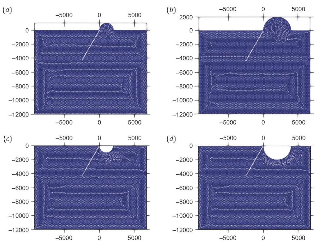
Fig. 2. Geometry of semi-circular hills and valleys. (a) – 1 km radius hill; (b) – 2 km radius hill; (c) – 1 km radius valley; (d) – 2 km radius valley.
Рис. 2. Геометрия полукруглых холмов и долин. (a) – холм радиусом 1 км; (b) – холм радиусом 2 км; (c) – долина радиусом 1 км; (d) – долина радиусом 2 км.
Table 1. Topographic features considered in this study
Таблица 1. Особенности рельефа, рассматриваемые в данной статье
|
Topo feature |
Hill |
Valley |
||
|
Semi-circle |
1 km (radius) |
2 km (radius) |
1 km (radius) |
2 km (radius) |
|
Gaussian |
1 km (3σ*) |
2 km (3σ) |
1 km (3σ) |
2 km (3σ) |
Note. *σ – standard deviation for a normal distribution.
Примечание. *σ – стандартное отклонение нормального распределения.
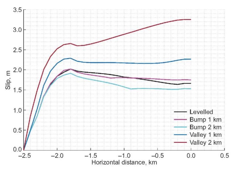
Fig. 3. Slip as a function of distance for upward (bump) and downward (valley) semi-circular topographic feature compared with that of flat topography (levelled).
Рис. 3. Смещение как функция расстояния для повышенных (холмы) и пониженных (долины) полукруглых форм рельефа в сравнении с плоским (ровным) рельефом.
Though the semi-circular features in topography are well described mathematically, naturally observed hills and valleys are more Gaussian-shaped (Fig. 4). All Gaussian profiles referred to herein are normal distributions. The equivalent of the radius of a semicircle, considered here, is half-width of Gaussian function covering 99.7 % confidence interval. Such a confidence interval is the same as six times the standard deviation (σ). So, the radius referred to in section 4.1 is 3σ. However, the largest amplification is observed for σ=1/3 valley in case of Gaussian topography, unlike that of semi-circular topography where the largest amplification was observed for a 2 km radius valley. Using the normalized Gaussian profile, this difference can be explained by the fact that the σ=1/3 Gaussian valley, exposed to the waves travelling from the up-dip rupture propagation, has a larger surface area than σ=2/3 Gaussian valley (Fig. 5).
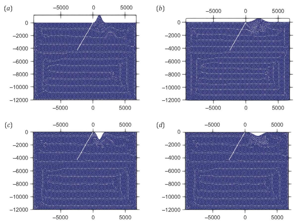
Fig. 4. Geometry of Gaussian hills and valleys.
(a) – 1 km half-width of a 99.7 % confidence interval hill; (b) – 2 km half-width of a 99.7 % confidence interval hill; (c) – 1 km half-width of a 99.7 % confidence interval valley; (d) – 2 km half-width of a 99.7 % confidence interval valley.
Рис. 4. Геометрия гауссовых холмов и долин.
(a) – холм полушириной 1 км с доверительным интервалом в 99.7 %; (b) – холм полушириной 2 км с дов. инт. в 99.7 %; (c) – долина полушириной 1 км с дов. инт. в 99.7 %; (d) – долина полушириной 2 км с дов. инт. в 99.7 %.
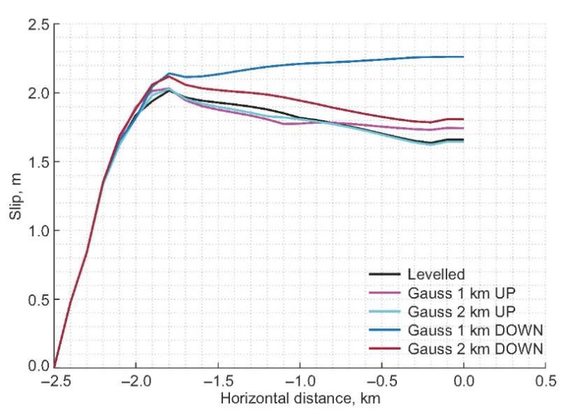
Fig. 5. Slip as a function of distance for upward (bump) and downward (valley) Gaussian topographic feature compared with that of flat topography (levelled).
Рис. 5. Смещение как функция расстояния для повышенных (холмы) и пониженных (долины) гауссовых форм рельефа в сравнении с плоским (ровным) рельефом.
To understand the slip amplification (or de-amplification) on the fault surface due to upward undulation (hill) ocurring at different distances, we use four models as shown in Fig. 6. This section addresses the effect of distance from hill to fault by considering a 1 km radius semi-circular hill located at 0 km, 2 km and 4 km distance from the tip of the fault. The variation in final slip with horizontal distance for all three cases is shown in Fig. 7, along with the final slip for the reference case. It can be observed in Fig. 7 that the free surface slip is decreasing if a hill-like feature is located far from the fault. It is also observed that peak slip occurs at nucleation patch for all four configurations. In comparison to a hill located at 0 km from the fault, the slip at the intersection of fault with a free surface is considerably less in the reference model, as well as in comparison to 2 km and 4 km distant hill-like feature models.
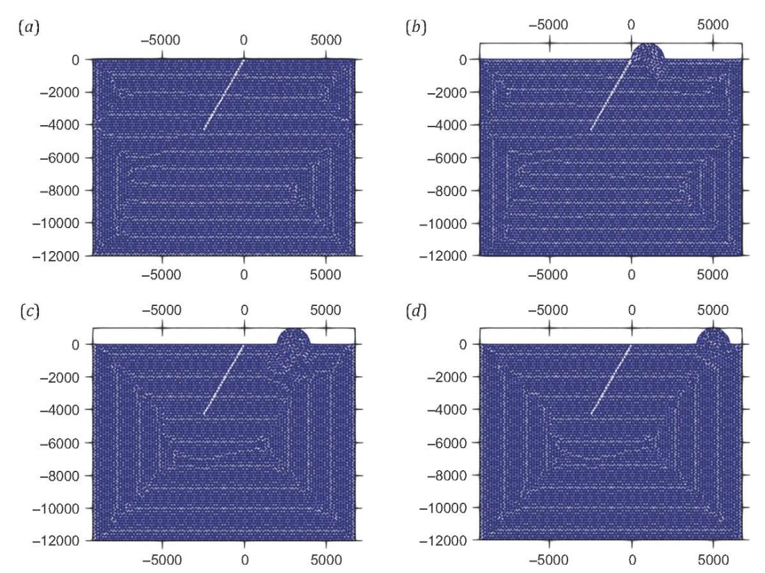
Fig. 6. Geometry of semi-circular 1 km radius hill located at distance 0 km (b), 2 km (c), and 4 km (d) from the intersection of fault with a free surface. (a) – reference case.
Рис. 6. Геометрия полукруглого холма радиусом 1 км, находящегося в 0 км (b), в 2 км (c) и в 4 км (d) от точки пересечения разлома со свободной поверхностью. (a) – базовая модель.
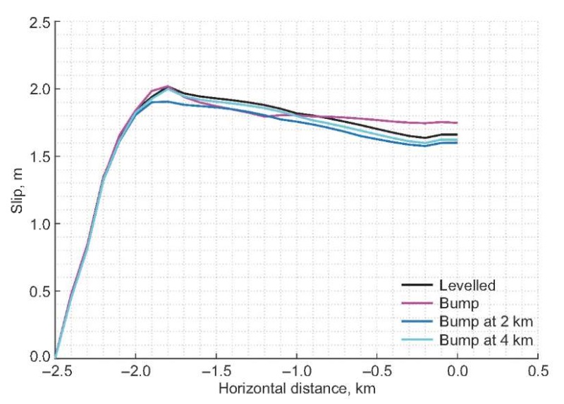
Fig. 7. Slip as a function of distance for upward semi-circular topographic feature (bump) located at 0, 2 and 4 km from the intersection of fault with a free surface compared with that of flat topography (levelled).
Рис. 7. Смещение как функция расстояния для повышенных полукруглых форм рельефа (холмы), находящихся в 0, 2 и 4 км от точки пересечения разлома со свободной поверхностью в сравнении с плоским (ровным) рельефом.
Unlike purely downward undulation (valley) cases, in topographic environments as those in Fig. 6, there are no potential edge-like features to cause wave reflections and slip amplification on fault surface due to the interference of edge-reflected waves. And this could be the main reason for little-observed amplification of slip for configurations shown in Fig. 6. Further, a trend in variation of slip value after nucleation patch for the case of a 4 km distant hill is the same as that for the reference case, thus depicting that the effect of topography will be insignificant if hill-like features form far from the intersection of fault with surface. As discussed, the hill-like feature with a 1 km radius at 0 km from the intersection of fault with surface shows a mixed pattern consisting of slip variation and horizontal distance patterns.
As shown in Fig. 8, the study of three configurations with a 1 km radius semi-circular downward undulation (valley) located at 0 km, 2 km, and 4 km from the intersection of fault with a free surface addresses the effect of distance on slip amplification. The final slip values from the numerical simulations for all three cases are compared with the reference case. The final slip on fault as function of a horizontal distance for the three configurations is shown in Fig. 9 along with the reference case. Unlike the case of semi-circular upward undulation (hill), the presence of semi-circular downward undulation (valley) amplifies the slip on fault for all three different valley locations. In Fig. 9 it can be observed that the slip amplification decreases linearly with increasing distance from valley to fault. The case with a valley-like feature at 0 km from the fault exhibits the maximum slip amplification as compared to the cases with 2- and 4-km distant valleys.
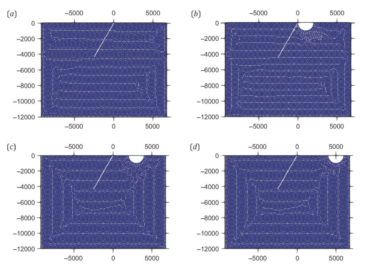
Fig. 8. Geometry of semi-circular 1 km radius valley located at distance 0 km (b), 2 km (c), and 4 km (d) from the intersection of fault with a free surface. (a) – reference case.
Рис. 8. Геометрия полукруглой долины радиусом 1 км, находящейся в 0 км (b), в 2 км (c), и в 4 км (d) от точки пересечения разлома со свободной поверхностью. (a) – базовая модель.
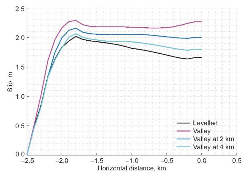
Fig. 9. Slip as a function of distance for downward semi-circular topographic feature (valley) located at 0, 2 and 4 km from the intersection of fault with a free surface compared with that of flat topography (levelled).
Рис. 9. Смещение как функция расстояния для пониженных полукруглых форм рельефа (долины), находящихся в 0, 2 и 4 км от точки пересечения разлома со свободной поверхностью в сравнении с плоским (ровным) рельефом.
Furthermore, the effect of fault-to-feature distance on slip amplification in downward undulation (valley) is more prominent than in upward undulation (hill). Except for valley located at 0 km from the fault, all the cases showed peak slip near nucleation patch on fault. The effect of interaction of edge-reflected waves is insignificant if the valley-like features are more distant and result in minimum amplification of slip on fault. The gap between the slip values of reference case and those of valley cases at the free surface intersection is larger than that at nucleation patch: in other words, the amplification of slip at the free surface intersection is more enhanced than at nucleation patch. Reason for this could be the reflected waves interacting with slip propagation at the free surface intersection rather than with slip propagation at nucleation patch which is located at a greater distance from the reflection-causing feature.
Since natural profiles of hills and valleys are more Gaussian-shaped and located at different distances in the proximity of fault, the effect of distance on slip amplification was studied with three models of Gaussian upward undulation (hill) with a half-width of 1 km and a 99.7 % confidence interval, located at 0 km, 2 km and 4 km from the fault as shown in Fig. 10. Fig. 11 shows the the plotted changes in fault slip values with horizontal distance for all the cases. As can be seen from Fig. 11, for the case of the hill 0 km distant from the fault, the amount of final slip on fault at the intersection with a free surface is larger than that for the reference case and two other cases. The slip values at nucleation patch are nearly the same for all the configurations and the peak slip occurred at nucleation patch in all four cases. Fig. 11 shows that the effect of hill-to-fault distance on slip amplification is insignificant if the distance is beyond a certain limit. As can be seen, slip as a function of horizontal distance is similar for reference case and for the case of the hill 4 km distant from the intersection of fault with a free surface.
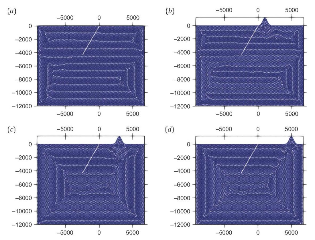
Fig. 10. Geometry of Gaussian 1 km half width of a 99.7 % confidence interval hill located at distance 0 km (b), 2 km (c), and 4 km (d) from the intersection of fault with a free surface. (a) – reference case.
Рис. 10. Геометрия гауссова холма полушириной 1 км с доверительным интервалом в 99.7 %, находящегося на расстоянии 0 (b), 2 (c) и 4 км (d) от точки пересечения разлома со свободной поверхностью. (a) – базовая модель.
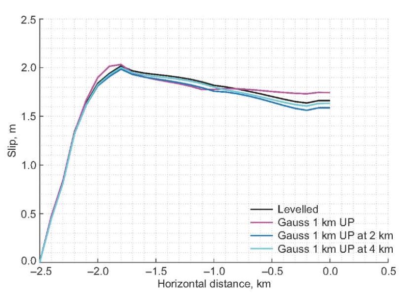
Fig. 11. Slip as a function of distance for upward Gaussian topographic feature (hill) located at 0, 2 and 4 km from the intersection of fault with a free surface compared with that of flat topography (levelled).
Рис. 11. Смещение как функция расстояния для повышенных гауссовых форм рельефа (холмы), находящихся на расстоянии 0, 2 и 4 км от точки пересечения разлома со свободной поверхностью в сравнении с плоским (ровным) рельефом.
Gaussian-shaped downward undulation (valley) 0 km, 2 km and 4km from the intersection of fault with a free surface, as shown in Fig. 12, was studied in order to understand the effect of distance on slip amplification. The final slip amounts from the numerical simulations are compared with reference case and shown in Fig. 13 as a function of horizontal distance. Unlike upward undulation, the Gaussian valley-like topography amplifies the slip on fault in all three cases, and the maximum amplification can be observed for the valley located at 0 km distance. As shown in Fig. 13, the amplification is less for the case of maximum fault-to-valley distance. Except for the valley located 0 km from the fault, peak slip near nucleation patch on fault is observed in all cases. It is clear, that the effect of distance on slip amplification is larger for the cases of downward Gaussian undulation than for the cases of upward undulation. For the case of a 4 km distant valley, the slip amplification started at a horizontal distance of 1 km from nucleation patch, whereas for other cases the amplification started immediately from the nucleation patch in up-dip direction. Except in the case of a 0 km distant valley, the peak slip values are observed near the free surface intersection.
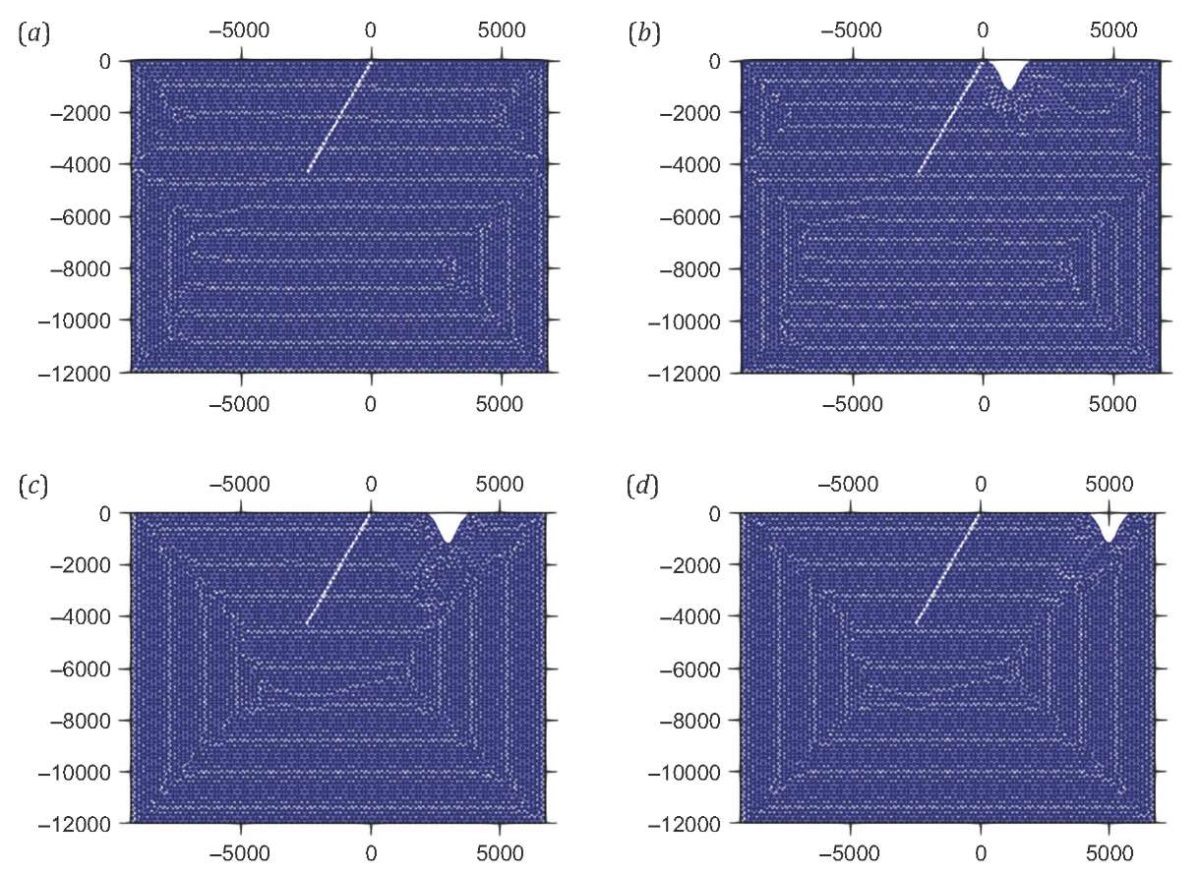
Fig. 12. Geometry of Gaussian 1 km half width of a 99.7 % confidence interval valley located at distance 0 km (b), 2 km (c), and 4 km (d) from the intersection of fault with a free surface. (a) – reference case.
Рис. 12. Геометрия гауссовой долины полушириной 1 км с доверительным интервалом в 99.7 %, находящейся на расстоянии 0 км (b), 2 км (c) и 4 км (d) от точки пересечения разлома со свободной поверхностью. (a) – базовая модель.
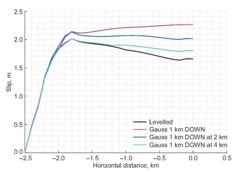
Fig. 13. Slip as a function of distance for downward Gaussian topographic feature (valley) located at 0, 2 and 4 km from the intersection of fault with a free surface compared with that of flat topography (levelled).
Рис. 13. Смещение как функция расстояния для пониженных гауссовых форм рельефа (долины), находящихся в 0, 2, и 4 км от точки пересечения разлома со свободной поверхностью в сравнении с плоским (ровным) рельефом.
A valley or a depression in the footwall of a dipping fault reaching free surface can be a curse, as there could be an amplification of slip near the intersection of a free surface with fault. Higher slip here is used as a proxy for larger damage in evaluating the curse or boon due to topographic feature. The curse could possibly be worsened by excavating deeper in the footwall, particularly with a profile that is near vertical on the side of a trough closer to the fault. Presence of a hill on footwall near the intersection of fault with a free surface can be a boon or a curse depending on the dimensions and location of the hill, while boon intensity is insignificant compared to the curse a valley can be. In the case of a valley, the effect of fault-to-hill or fault-to-valley distance on slip amplification is larger than that in the case of a hill. The major limitations of the study include the simplicity of the relief models which only have a hill or a valley at a time, whereas in reality both positive and negative relief forms do exist together in the fault zone. This paper can be extended to evaluate the effect of multiple topographic features as boon or curse for other dip angles and different initial conditions.
The authors thank Indian Institute of Tropical Meteorology (IITM) for giving access to Aaditya HPC Supercomputing resources to run PyLith.
Both authors made an equivalent contribution to this article, read and approved the final manuscript.
Both authors declare that they have no conflicts of interest relevant to this manuscript.
1. Aagaard B., Kientz S., Knepley M., Somala S., Strand L., Williams C., 2010. PyLith User Manual, Version 1.5.0. Computational Infrastructure of Geodynamics, Pasadena, CA, USA, 224 p.
2. Aagaard B.T., Knepley M.G., Williams C.A., 2013. A Domain Decomposition Approach to Implementing Fault Slip in Finite-Element Models of Quasi-Static and Dynamic Crustal Deformation. Journal of Geophysical Research: Solid Earth 118 (6), 3059–3079. https://doi.org/10.1002/jgrb.50217.
3. Andrews D.J., 1976. Rupture Velocity of Plane Strain Shear Cracks. Journal of Geophysical Research 81 (32), 5679–5687. https://doi.org/10.1029/JB081i032p05679.
4. Aochi H., Fukuyama E., Matsu’ura M., 2000. Spontaneous Rupture Propagation on a Non-Planar Fault in 3-D Elastic Medium. Pure and Applied Geophysics 157, 2003–2027. https://doi.org/10.1007/PL00001072.
5. Benjemaa M., Glinsky-Olivier N., Cruz-Atienza V.M., Virieux J., 2009. 3-D Dynamic Rupture Simulations by a Finite Volume Method. Geophysical Journal International 178 (1), 541–560. https://doi.org/10.1111/j.1365-246X.2009.04088.x.
6. Benjemaa M., Glinsky-Olivier N., Cruz-Atienza V.M., Virieux J., Piperno S., 2007. Dynamic Non-Planar Crack Rupture by a Finite Volume Method. Geophysical Journal International 171 (1), 271–285. https://doi.org/10.1111/j.1365-246X.2006.03500.x.
7. Chen X., Zhang H., 2006. Modelling Rupture Dynamics of a Planar Fault in 3-D Half Space by Boundary Integral Equation Method: An Overview. Pure and Applied Geophysics 163, 267–299. https://doi.org/10.1007/s00024-005-0020-z.
8. Das S., Aki K., 1977. A Numerical Study of Two-Dimensional Spontaneous Rupture Propagation. Geophysical Journal International 50 (3), 643–668. https://doi.org/10.1111/j.1365-246X.1977.tb01339.x.
9. Day S.M., Dalguer L.A., Lapusta N., Liu Y., 2005. Comparison of Finite Difference and Boundary Integral Solutions to Three-Dimensional Spontaneous Rupture. Journal of Geophysical Research: Solid Earth 110 (В12). https://doi.org/10.1029/2005JB003813.
10. Day S.M., Gonzalez S.H., Anooshehpoor R., Brune J.N., 2008. Scale-Model and Numerical Simulations of Near-Fault Seismic Directivity. Bulletin of the Seismological Society of America 98 (3), 1186–1206. https://doi.org/10.1785/0120070190.
11. Ely G.P., Day S.M., Minster J.-B., 2009. A Support-Operator Method for 3-D Rupture Dynamics. Geophysical Journal International 177 (3), 1140–1150. https://doi.org/10.1111/j.1365-246X.2009.04117.x.
12. Ely G.P., Day S.M., Minster J.-B., 2010. Dynamic Rupture Models for the Southern San Andreas Fault. Bulletin of the Seismological Society of America 100 (1), 131–150. https://doi.org/10.1785/0120090187.
13. Fukuyama E., Madariaga R., 1998. Rupture Dynamics of a Planar Fault in a 3D Elastic Medium: Rate- and Slip-Weakening Friction. Bulletin of the Seismological Society of America 88 (1), 1–17. https://doi.org/10.1785/BSSA0880010001.
14. Harris R.A., Barall M., Archuleta R., Dunham E., Aagaard B., Ampuero J.P., Bhat H., Cruz-Atienza V. et al., 2009. The SCEC/USGS Dynamic Earthquake Rupture Code Verification Exercise. Seismological Research Letters 80 (1), 119–126. https://doi.org/10.1785/gssrl.80.1.119.
15. Hok S., Fukuyama E., 2011. A New BIEM for Rupture Dynamics in Half-Space and Its Application to the 2008 Iwate-Miyagi Nairiku Earthquake. Geophysical Journal International 184 (1), 301–324. https://doi.org/10.1111/j.1365-246X.2010.04835.x.
16. Huang H., Zhang Z., Chen X., 2018. Investigation of Topographical Effects on Rupture Dynamics and Resultant Ground Motions. Geophysical Journal International 212 (1), 311–323. https://doi.org/10.1093/gji/ggx425.
17. Ida Y., 1972. Cohesive Force across the Tip of a Longitudinal-Shear Crack and Griffith’s Specific Surface Energy. Journal of Geophysical Research 77 (20), 3796–3805. https://doi.org/10.1029/JB077i020p03796.
18. Kaneko Y., Lapusta N., 2010. Supershear Transition Due to a Free Surface in 3-D Simulations of Spontaneous Dynamic Rupture on Vertical Strike-Slip Faults. Tectonophysics 493 (3–4), 272–284. https://doi.org/10.1016/j.tecto.2010.06.015.
19. Kaneko Y., Lapusta N., Ampuero J.-P., 2008. Spectral Element Modeling of Spontaneous Earthquake Rupture on Rate and State Faults: Effect of Velocity-Strengthening Friction at Shallow Depths. Journal of Geophysical Research: Solid Earth 113 (В9). https://doi.org/10.1029/2007JB005553.
20. Madariaga R., 1976. Dynamics of an Expanding Circular Fault. Bulletin of the Seismological Society of America 66 (3), 639–666. https://doi.org/10.1785/BSSA0660030639.
21. Oglesby D.D., Archuleta R.J., Nielsen S.B., 2000a. Dynamics of Dip-Slip Faulting: Explorations in Two Dimensions. Journal of Geophysical Research: Solid Earth 105 (В6), 13643–13653. https://doi.org/10.1029/2000JB900055.
22. Oglesby D.D., Archuleta R.J., Nielsen S.B., 2000b. The Three-Dimensional Dynamics of Dipping Faults. Bulletin of the Seismological Society of America 90 (3), 616–628. https://doi.org/10.1785/0119990113.
23. Parla R., Shanmugasundaram B., Somala S.N., 2022. Basin Effects on the Seismic Fragility of Steel Moment Resisting Frames Structures: Impedance Ratio, Depth, and Width of Basin. International Journal of Structural Stability and Dynamics 22 (09), 2250108. https://doi.org/10.1142/S0219455422501085.
24. Parla R., Somala S.N., 2022a. Numerical Modeling of Quaternary Sediment Amplification: Basin Size, ASCE Site Class, and Fault Location. International Journal of Geotechnical Earthquake Engineering 13 (1), 1–20. https://doi.org/10.4018/IJGEE.303589.
25. Parla R., Somala S.N., 2022b. Seismic Ground Motion Amplification in a 3D Sedimentary Basin: Source Mechanism and Intensity Measures. Journal of Earthquake and Tsunami 16 (4), 1793–7116. https://doi.org/10.1142/S1793431122500087.
26. Somala S.N., Parla R., Mangalathu S., 2022. Basin Effects on Tall Bridges in Seattle from M9 Cascadia Scenarios. Engineering Structures 260 (1), 114252. https://doi.org/10.1016/j.engstruct.2022.114252.
27. Tago J., Cruz‐Atienza V.M., Virieux J., Etienne V., Sánchez-Sesma F.J., 2012. A 3D Hp-Adaptive Discontinuous Galerkin Method for Modeling Earthquake Dynamics. Journal of Geophysical Research: Solid Earth 117, (B9). https://doi.org/10.1029/2012JB009313.
28. Xu J., Zhang H., Chen X., 2015. Rupture Phase Diagrams for a Planar Fault in 3-D Full-Space and Half-Space. Geophysical Journal International 202 (3), 2194–2206. https://doi.org/10.1093/gji/ggv284.
29. Zhang H., Chen X., 2006a. Dynamic Rupture on a Planar Fault in Three-Dimensional Half Space – I. Theory. Geophysical Journal International 164 (3), 633–652. https://doi.org/10.1111/j.1365-246X.2006.02887.x.
30. Zhang H., Chen X., 2006b. Dynamic Rupture on a Planar Fault in Three‐Dimensional Half-Space – II. Validations and Numerical Experiments. Geophysical Journal International 167 (2), 917–932. https://doi.org/10.1111/j.1365-246X.2006.03102.x.
31. Zhang Z., Xu J., Chen X., 2016. The Supershear Effect of Topography on Rupture Dynamics. Geophysical Research Letters 43 (4), 1457–1463. https://doi.org/10.1002/2015GL067112.
32. Zhang Z., Zhang W., Chen X., 2014. Three-Dimensional Curved Grid Finite-Difference Modelling for Non-Planar Rupture Dynamics. Geophysical Journal International 199 (2), 860–879. https://doi.org/10.1093/gji/ggu308.
Hyderabad 502285
Hyderabad 502285
Parla R., Somala S.N. INFLUENCE OF HILLS AND VALLEYS ON FREE SURFACE SLIP AMPLIFICATION IN DYNAMIC RUPTURE ON A DIPPING FAULT. Geodynamics & Tectonophysics. 2024;15(4):0777. https://doi.org/10.5800/GT-2024-15-4-0777. EDN: ELARBH


Editor-in-Chief
Sklyarov E.V.664033, Irkutsk, Lermontova St., 128,
IEC SB RAS Institute of the Earth's crust
E-mail.: gt@crust.irk.ru
tel.: 8 3952 425422
Processing of personal data


