


Contents
Scroll to:
https://doi.org/10.5800/GT-2024-15-4-0772
EDN: FWESLM
Scroll to:
Bandar Lampung City is located at the southeastern tip of Sumatra Island, an area highly prone to earthquake and tsunami disasters. Along the Sumatra Island, there are seismic faults stretching along the Bukit Barisan Mountains. In the Bandar Lampung region, one of these faults is the Panjang Lampung fault. Gravity methods are commonly used to identify subsurface structures based on variations in rock density. This study aims to identify the subsurface structure of Bandar Lampung City based on gravity anomaly modeling, both 2D and 3D models. The research consists of three main stages: data correction, data processing including spectrum analysis, moving average, second vertical derivative analysis, and subsurface structure modeling. The complete Bouguer anomalies in the study area range from 41.9 mGal to 73.3 mGal. Modeling results indicate the presence of structures such as the Panjang Lampung fault in the Northeast and a graben in the Central region, verified through SVD analysis and geological information. The existence of the Panjang Lampung fault, classified as an active fault, along with volcanic pyroclastic rocks and significant sediment layers in the central region, makes the research area potentially susceptible to the impact of amplification in the event of an earthquake disaster.
Dani I., Zaenudin A., Hutomo A.I., Yuniza N. ANALYSIS OF SUBSURFACE STRUCTURE OF BANDAR LAMPUNG CITY BASED ON GRAVITY ANOMALIES. Geodynamics & Tectonophysics. 2024;15(4):0772. https://doi.org/10.5800/GT-2024-15-4-0772. EDN: FWESLM
Bandar Lampung is the capital of Lampung Province which is located on the southeastern tip of Sumatra Island, Indonesia. Geographically, this city is located in the southwest of Sumatra Island, Indonesia, at 5°26' latitude south and 105°15' longitude east. In January 2022, the area of Bandar Lampung City, covering around 118.5 km2, was divided into 20 sub-districts and 126 villages. According to data from the Ministry of Home Affairs, the population of Bandar Lampung City reached 1096936 people in mid-2023 [Bandar Lampung…, 2023]. Administratively, this city is bordered on the north to east by Lampung Selatan Regency, on the south by the Sunda Strait, and on the west by Pesawaran Regency.
The geomorphological character of Bandar Lampung City is influenced by its location on the coast of the Lampung Bay and variations in elevation and land slopes from the coast inland [Mulyasari et al., 2019]. The city lies at elevations of 0 to 700 m above sea level with topography involving coastal areas, hilly areas around northern Betung Bay, and undulating highlands around western Tanjung Karang as well as small islands in the south. Rivers such as Way Balau, Way Halim, Way Awi, Way Kuripan, Way Simpur, Way Garuntang, and Way Kupang flow through the city. Some areas of Bandar Lampung City are hilly such as Mount Kunyit, Mount Bakung, Mount Mastur and some other hills. This topography includes flat to gently sloping and steep to very steep land, accounting for about 60 %, 35 %, and 4 % of the total area, respectively [Bandar Lampung , 2023].
Based on the geological map of Tanjung Karang sheet [Mangga et al., 1993], the city of Bandar Lampung is located in the Mount Kasih complex [Rustadi, Rananda, 2020]. This complex consists of metamorphic rocks which are interpreted as the oldest geological formations [Setiawan et al., 2013; Akinin, Zhulanova, 2016]. The rocks involved include schist, gneiss, quartzite, and marble, which are exposed due to the erosion of the overlying Quaternary rocks and tectonics acting upon limestone sediments. They are assigned an Early Carboniferous or older age and they likely represent the crystalline basement rocks that form the foundation for a wide initial sedimentary basin in the back-arc region. The Lampung formation (Qtl) dominates most of the Tanjung Karang sheet and consists of rhyolite-tuff and volcaniclastic tuff rocks. Volcanic activity related to the subduction of the Indian Ocean plate occurred along the mountain range arc during the Tertiary period, resulting in tuff rocks, lava, and volcanic breccia with a basaltic rhyolite composition. Depositional processes during the Holocene contributed to the formation of alluvial deposits, limestone, and swamp areas [Salisbury et al., 2012].
The tectonic activity of Lampung province is largely influenced by the subduction zone, which makes it highly prone to earthquakes and tsunamis [Susilorini et al., 2021]. This is due to its proximity to active tectonic plate boundaries, specifically the convergence of the Eurasian, Indo-Australian, and Pacific plates around the Indian Ocean [Elliott et al., 2016]. Specifically, Bandar Lampung City is located along the subduction zone in the western part of Sumatra Island, where the Indo-Australian plate subducts beneath the Eurasian Plate [Gao et al., 2020] which can cause earthquakes. Earthquakes are natural events that occur due to the sudden release of energy from within the Earth’s crust [Nielsen et al., 2016; Calais et al., 2016]. These events cause vibrations and shaking on the Earth’s surface [Elliott et al., 2020; Ali U., Ali S.A., 2020]. Meanwhile, subduction of plates in the Indian Ocean can cause the release of energy through faults parallel to the edges of oceanic plates, thereby triggering tsunamis [Rubin et al., 2017; Paris et al., 2020].
There are several active faults in Bandar Lampung area, among which one of the main ones is the Panjang Lampung fault [Siringoringo et al., 2023; Iqbal et al., 2023]. In its history, in 1913, the Panjang Lampung fault has experienced significant earthquakes with a magnitude of around 7 on the Richter scale, occurring at depths of 20–40 km [Naryanto, 2008; Vickers, 2013]. Due to the probability of occurrence of earthquakes in this research area, there is a potential risk of earthquake wave amplification, similar to what occurred in Yogyakarta in 2006 [Diambama et al., 2019]. This research aims to analyze the geological structure of Panjang Lampung for seismic hazard assessment.
The distribution of the rock density can cause anomalies in gravity, which can help depict the geological structure beneath the Earth’s surface to significant depths [Zaenudin et al., 2020; Ombati et al., 2022]. Therefore, in order to understand the fault patterns, geological structures, and types of rocks that may be succeptable to earthquakes and amplification in this research area, a study of the subsurface geological structure will be conducted using gravity methods. In this study, 2D forward modeling and 3D inversion will be performed based on the results of residual anomalies, supported by Second Vertical Derivative (SVD) analysis and 3D inversion.
Gravity data measurements were carried out in 2017 at 56 points spaced throughout the city of Bandar Lampung. The distance between measurement stations ranges from 600 to 1000 m with topographic variations ranging from 0 to 700 meters above mean sea level. Areas with low elevation are generally in the south, while undulating highland areas are in the west, east and north. All data is measured above the surface without using satellite data.
The data processing stages have begun with correcting the instrument readings, namely tide and drift corrections. The next step includes latitude and free air corrections. To find the surface density, use is made of the Parasnis method which is then followed by the Bouguer correction [Parasnis, 1986], thus obtaining the complete Bouguer anomaly value in the research area. Processing involves complete Bouguer anomaly data, followed by spectral analysis on 4 tracks using Fast Fourier Transform (FFT). The result is the spatial change from distance to spatial frequency, which is then used to determine the cut-off value. The window width is determined to separate regional anomalies and residuals using a moving average filter. Residual anomalies are analyzed by the SVD method using the Elkins operator [Elkins, 1951] and thus provide structural information on the research area for additional subsurface modeling.
The modeling carried out is 2D and 3D modeling. Forward 2D modeling is performed using the Oasis Montaj software, by drawing lines or making slices in areas showing anomalies. This modeling is based on the availability of seismic transects in the study area. The modeling results show correlation between gravity anomaly graphs, magnetic anomaly graphs, and subsurface cross-sections from the seismic data. 3D inverse modeling is carried out based on models directly produced from the data, focusing on residual anomaly data and density parameters obtained from geological information in the study area.
The flow diagram used in this study shown in Fig. 1.
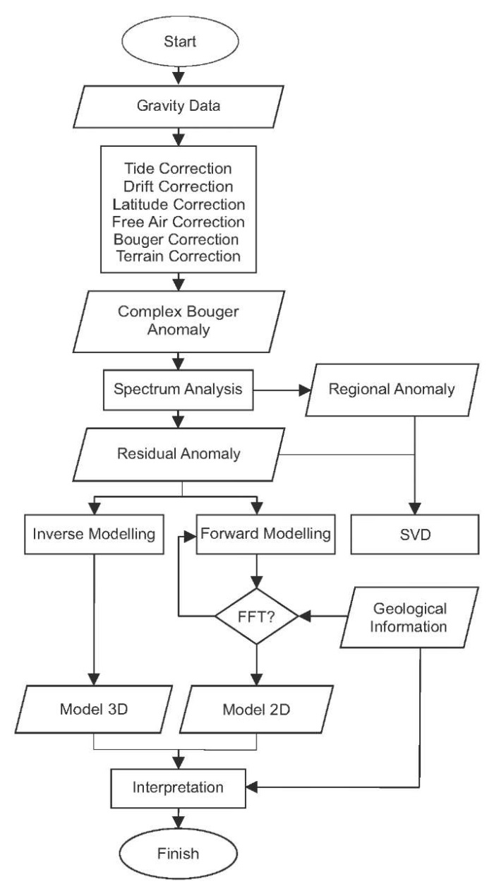
Fig. 1. Flow diagram.
Рис. 1. Блок-схема.
To obtain the complete Bouguer anomaly, corrections are needed for the data to remove the effects that were observed during the measurement. This study uses an average surface density of 2388.4 kg/m3, which is the average density calculated by the Parasnis method. The results of the correction calculations on the gravity data for the research area can be seen in Fig. 2.
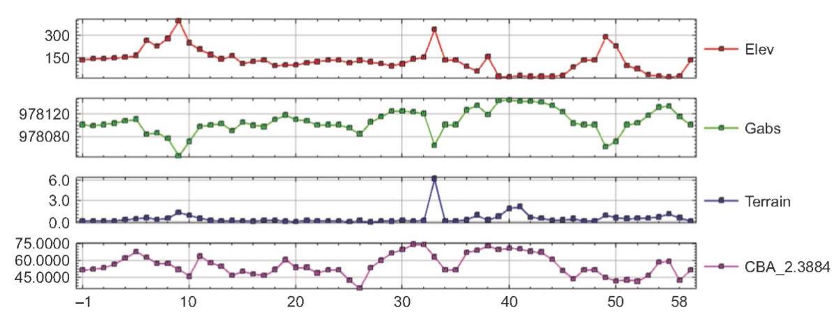
Fig 2. Gravity data correction results.
Рис. 2. Результаты коррекции гравитационных данных.
Based on the correction results, Fig. 2 shows the elevation value graph (red), observed G value (green), field correction result (blue), and Complete Bouguer Anomaly or CBA value (purple). In the field correction result, there is a relatively high correction value of 6.207 mGal at point BL-40. This result is influenced by the extreme topographic conditions around the measurement point. Then, in the green-colored graph (g. observed), it can be seen that it is inversely proportional to the blue-colored graph (elevation). Therefore, it can be concluded that the gravity value will decrease as the elevation of the measurement point increases.
After performing the necessary corrections on the above gravitational force, the next step is to calculate the complete Bouguer anomaly value for the research area, which can be seen in Fig. 3 (bottom).
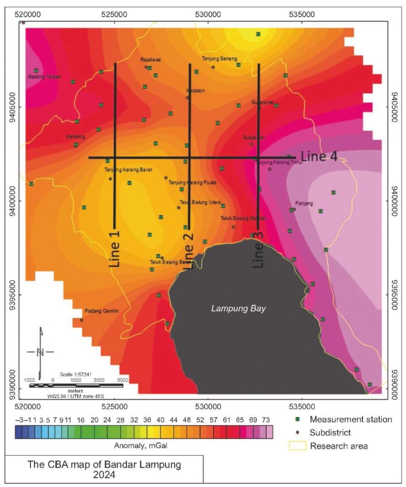
Fig. 3. Complete Bouguer anomaly map with profile lines
for determining regional and residual anomaly depths.
Рис. 3. Карта полной аномалии Буге с линиями профиля
для определения глубины региональных и остаточных аномалий.
On the contour map of the complete Bouguer anomaly in the research area, 4 profile lines were sliced as shown in Fig. 3. To determine the depth of shallow anomalies and deep anomalies, an analysis of the spectrum was conducted, where the log power spectrum (Ln A) against frequency is represented by the slope value (gradient) as seen in Fig. 4. Table 1 shows the average values for the estimated regional depth of 3000 m, residual depth of 222 m, and an average KC value of 0.00118 with an average window width of 10.6. Since the value of n must be odd, the value used to separate the regional and residual anomalies is rounded up to 11.
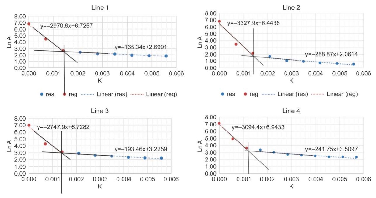
Fig. 4. Spectrum analysis chart on Line 1–4.
Рис. 4. Диаграммы спектрального анализа для линий 1–4.
Table 1. Spectrum analysis results
Таблица 1. Результаты спектрального анализа
|
Line |
KC |
Window width |
Depth, m |
|
|
Reginal |
Residual |
|||
|
1 |
0.0012 |
10.35 |
2971 |
165 |
|
2 |
0.0012 |
10.38 |
3328 |
289 |
|
3 |
0.0012 |
10.48 |
2748 |
194 |
|
4 |
0.0011 |
11.42 |
3094 |
242 |
|
Average |
0.0012 |
10.64 |
3035 |
222 |
For Line 1, the estimated regional depth is 2970 m; the residual depth is 165 m, with a KC wave value of 0.001212 and a window width of 10.36. Moving on to Line 2, the estimated regional depth is 3327 m, the residual depth is 288 m, with a KC wave value of 0.00121 and a window width of 10.38. For Line 3, the estimated regional depth is 3094 m; the residual depth is 241 m, with a KC wave value of 0.001199 and a window width of 11.418. Lastly, for Line 4, the estimated regional depth is 3094 m; the residual depth is 241 m, with a KC wave value of 0.0011 and a window width of 11.418.
Based on the spectrum analysis conducted, the estimated regional depth, residual depth, and KC (cutoff) wave value can be determined for each profile. The estimated regional depth indicates the depth of the basement, while the residual depth indicates the boundary between the basement and sedimentary rocks. The intersection value of the gradient between the residual and regional values is defined as the KC wave value, which will be used in determining the window width in the moving average process. The window width value is obtained using the formula 2π/ksΔx, where KC is the cutoff value and ∆x is the spacing.
Regional anomaly in Fig. 5, a is obtained from the processing of moving average filter on the complete Bouguer anomaly using Surfer software. This method is performed using the results of spectrum analysis based on the window width value obtained, n=11. Therefore, the residual anomaly is obtained by subtracting the complete Bouguer anomaly from the regional anomaly. The previous result obtained from the spectrum analysis for the average depth of the regional anomaly was 3000 m. The result of residual anomaly separation in Fig. 5, b is the result of subtraction between the complete Bouguer anomaly and the regional anomaly obtained from the spectrum analysis.
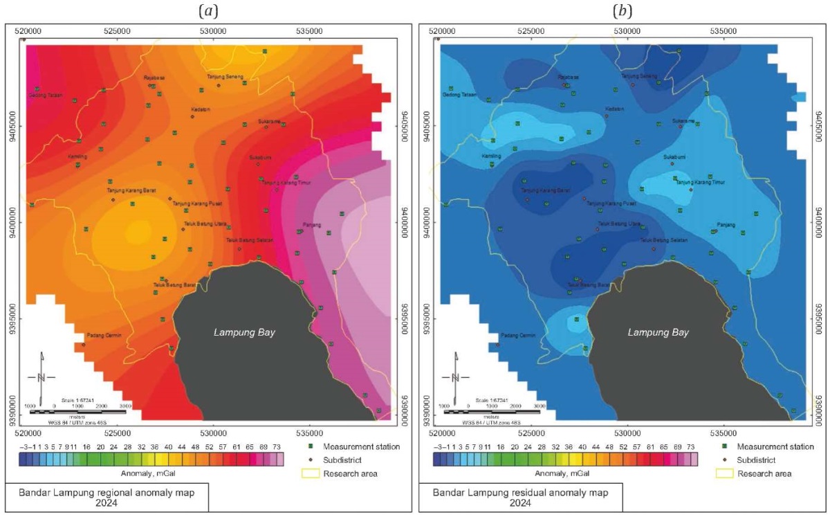
Fig. 5. Contour map of regional gravity anomaly
filtered with a window width and height of 11×11 (a)
and contour map of residual gravity anomaly (b).
Рис. 5. Карта региональной гравитационной аномалии с размером окна 11×11 (a)
и карта остаточной гравитационной аномалии (b).
The SVD analysis on this regional anomaly was conducted using the low pass filter [Kumar et al., 2018]. The results of the SVD analysis performed on the regional anomaly and residual anomaly of the study area can be seen in Fig. 6, a, c. The results obtained by using calculation operator on the residual anomaly are shown in Fig. 6, b. The black line represents the SVD value of 0. Based on this SVD value of 0, a selection is made based on the straightness indicated by the white line, as shown in Fig. 6, d.
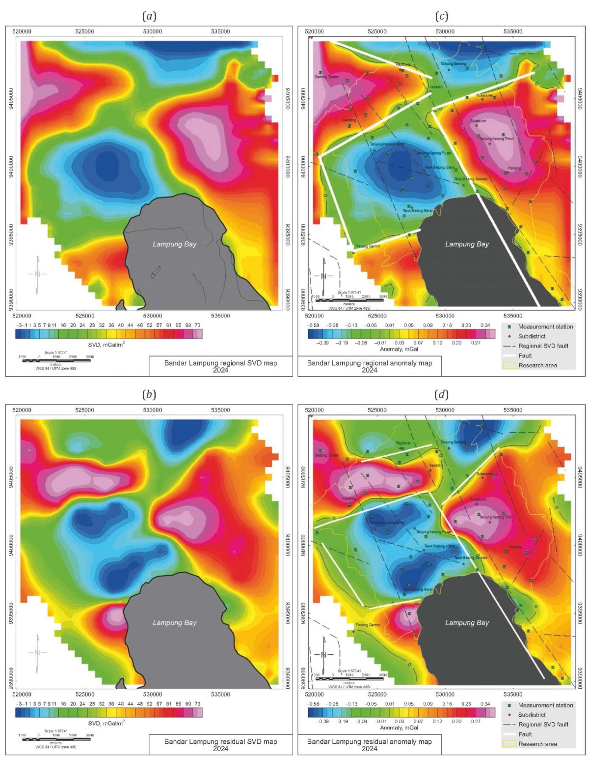
Fig. 6. Regional second vertical derivative map (a),
residual second vertical derivative map (b),
and fault indication map based on SVD analysis of regional (c) and residual anomalies (d).
Рис. 6. Региональная карта вторых вертикальных производных (a),
карта остатков для вторых вертикальных производных (b)
и карта с обозначениями разломов, составленная на основе анализа
вторых вертикальных производных для региональных (c) и остаточных (d) аномалий.
Modeling subsurface is conducted on two lines that intersect the main structure in the study area. The created tracks can be seen in Fig. 7. The forward 2D modeling is performed using Oasis Montaj software [Grandis, Dahrin, 2017].
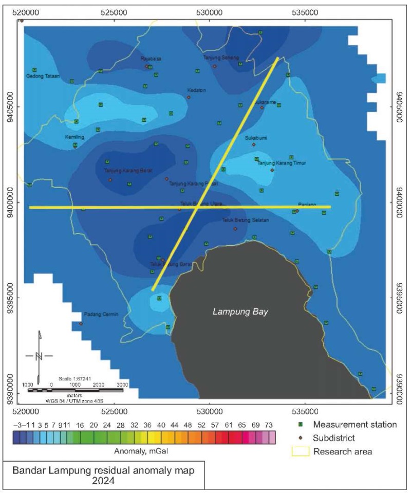
Fig. 7. Slicing forward modelling path map.
Рис. 7. Нарезка карты прямого моделирования.
The backward modeling (inversion) is a modeling process that estimates the distribution of density and susceptibility beneath the surface [Lücke, Arroyo, 2015], which can be seen in Fig. 8. This process is done using the VOXI menu in Oasis Montaj software, with input data in the form of residual anomalies, aiming to obtain an output in the form of a 3D model of the study area that approximates the actual conditions. The model is created by inputting parameters such as Xmin, Xmax, Ymin, Ymax, Zmin, Zmax, with a block size of 500×500×250. Then, the results of this inversion modeling are correlated with the two tracks in the previous forward 2D modeling, with the aim of highlighting the similarities in geological structures between the forward modeling and the 3D modeling.
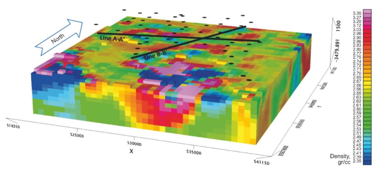
Fig. 8. Density distribution model from 3D inversion results.
Рис. 8. Модель распределения плотности,
основанная на результатах 3D инверсии данных.
The results of the 3D inversion are sliced along the same tracks as the tracks in the forward modeling, which can be seen in Fig. 9, d and Fig. 10, d. The 3D inversion modeling results show density contrasts that indicate the presence of a graben structure, which is also confirmed by the 2D forward modeling results. In addition, the 3D inversion model can also show the response of granite intrusions (Tmgr) in the study area.
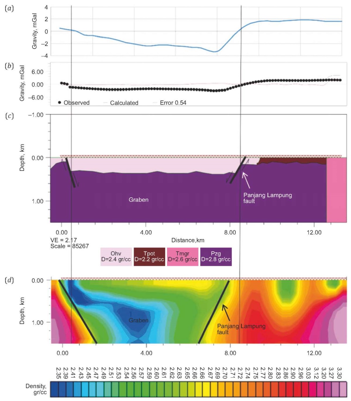
Fig. 9. Interpretation of the subsurface model Line A-A’.
(a) – calculated response of SVD anomalies;
(b) – observed response of SVD anomalies;
(c) – 2D modeling result;
(d) – 3D inversion model slice result.
Рис. 9. Интерпретация модели подземного пространства, линия A-A’.
(a) – расчетная реакция аномалий вторых вертикальных производных;
(b) – наблюдаемая реакция аномалий вторых вертикальных производных;
(c) – результат 2D-моделирования;
(d) – результат нарезки модели 3D-инверсии.
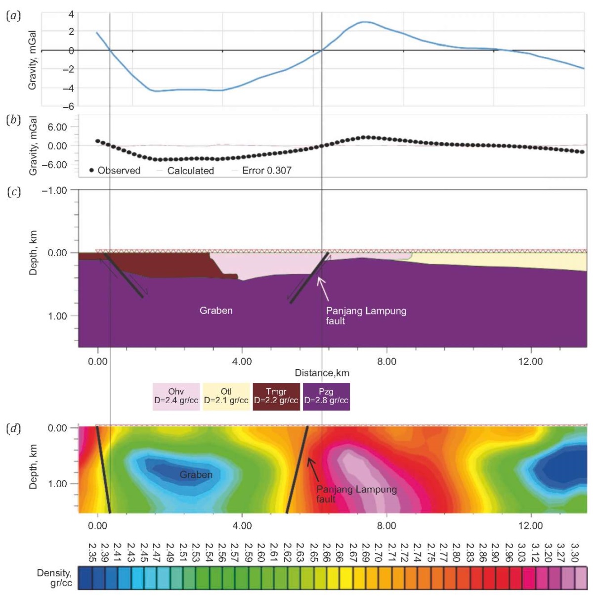
Fig. 10. Interpretation of the subsurface model Line B-B’.
(a) – calculated response of SVD anomalies;
(b) – observed response of SVD anomalies;
(c) – 2D modeling result;
(d) – 3D inversion model slice result.
Рис. 10. Интерпретация модели подземного пространства, линия B-B’.
(a) – расчетная реакция аномалий вторых вертикальных производных;
(b) – наблюдаемая реакция аномалий вторых вертикальных производных;
(c) – результат 2D-моделирования;
(d) – результат нарезки модели 3D-инверсии.
Bouguer anomaly is the difference between the measured gravity force value and the theoretical gravity force value. The value of Bouguer anomaly is the result of superposition of regional anomaly (deep gravity response) and residual anomaly (shallow gravity response). In the process of reducing the data due to the influence of mass below and around the measurement point to obtain the Bouguer anomaly value, the calculation of average surface density is first performed using the Parasnis or Nattelton method [Maunde et al., 2017].
The complete Bouguer anomaly contour is the result of 500 m gridding. The spacing interval is determined based on an average spacing of 1000 m between the measurement points. Therefore, the complete Bouguer anomaly data are gridded with a spacing of 500 m. In Fig. 3, the range of anomaly values is divided into three parts: high anomaly, moderate anomaly, and low anomaly, with a range of values between 41.9 and 73.3 mGal, which represents the response of rock density variations in the study area. The distribution of high anomalies is in the western and eastern parts of the study area, indicated by the color ranging from orange to pink, with a range of values from 59.5 to 73.3 mGal. The distribution of low anomalies is found in the northern and southwestern parts of the complete Bouguer anomaly map, indicated by dark-to-light-blue color, with a range of anomaly values between 41.9 and 50 mGal. As for the moderate anomalies, they are located between the distribution of high and low anomalies, indicated by the color ranging from dark green to yellow, with a range of anomaly values between 50 and 59.5 mGal.
The slicing results will be involved in spectrum analysis, which is performed using Fourier transform to convert gravity data from spatial domain to frequency domain using Matlab software. The Fourier transform process will produce real and imaginary values, where the real value represents the x-axis and the imaginary value represents the y-axis. The spectrum analysis is shown in the the graph for relationship between ln(A) and k, where ln(A) is obtained from , and k is obtained from 2πf. The frequency value is obtained by dividing the data sequence by the number of data points multiplied by the spacing.
In spectrum analysis, the sources located deep beneath the surface will show low-frequency values, while those sources originating from shallow depths will exhibit high-frequency values. This is because the rocks deep beneath the surface tend to be homogeneous and have consistent densities, whereas shallow sources have more varied rock compositions, resulting in different density values.
Regional anomalies have low frequency, but high wave amplitude, where the anomaly response is assumed to originate from rocks at large and more homogeneous depths with high density values. Based on Fig. 5, a, the contour of the regional anomaly obtained ranges from 44 to 73 mGal, with a contour pattern that is almost the same as the complete Bouguer anomaly contour. Based on the spectrum analysis, the residual anomaly (see Fig. 5, b) is found at a depth of 222 m with a maximum depth of up to 3000 m. On the residual anomaly map, high anomalies can be seen in the eastern and western parts of the study area, while low anomalies are in its northern and southern parts. The resulting residual anomalies range from –5 to 5 mGal.
The result of the SVD analysis is an inferred fault structure that is superimposed on the structures in the geological map (Fig. 11). Based on the geological map of the study area, the presence of southwest-northeast fault structures can be validated with the results of the SVD analysis showing two faults which have relatively similar orientations but do not intersect.
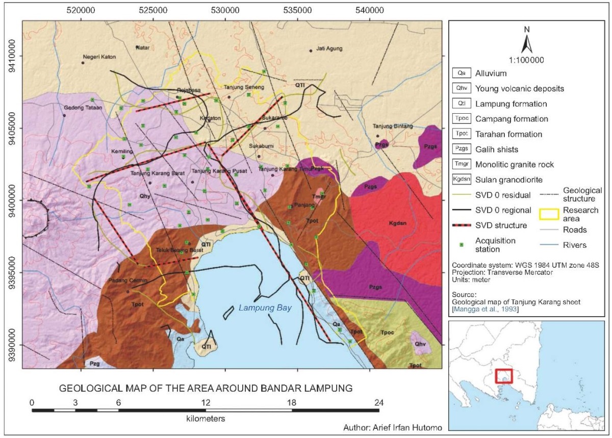
Fig. 11. Geological overlay map with SVD analysis results.
Рис. 11. Геологическая оверлейная карта
с результатами анализа вторых вертикальных производных.
In addition to these two southwest-northeast faults, the SVD analysis also indicates faults having relative east-west orientation. Therefore, in connection with the residual anomaly lows in the central fault-bounded part it can be inferred that there is a graben structure in the study area. The indications of new faults in the study area obtained from the SVD analysis are further confirmed by geological events that show surface faulting evidence such as steep topography in the form of hills and rivers in the study area, as seen in the overlay of the DEM map with the SVD-generated faults and the geological faults (Fig. 12).
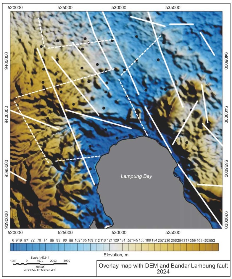
Fig. 12. Overlay map with DEM and fault indication.
Рис. 12. Оверлейная карта c ЦМР и обозначением разлома.
The basic principle of the forward modeling process is trial and error to achieve alignment between theoretical data and field data. In line with the goal of this research, which is to obtain a subsurface model to validate the structure in the study area, the modeling is done by combining existing information, including geological information about surface geology, geological structures, and stratigraphy in the study area. Additionally, information from gravity data includes the complete Bouguer anomaly, spectrum analysis, residual and regional anomalies, and the results of SVD analysis. The integration of this information is expected to result in a subsurface model with minimal ambiguity. Gravity information is obtained from spectrum analysis, where it is known that the depth of the anomaly is 3 km. This depth will be used as the boundary between the residual anomaly and the regional anomaly (basement) in the modeling process. Based on SVD analysis, it is known that there are fault structures in the study area that can be validated with the geological map.
Fig. 9, c shows the results of the subsurface model in Line A-A’ (west-east). Based on the surface geology, Line A-A’ passes through two fault structures, two formations exposed on the surface, namely the young volcanic deposits (Qhv) and the Tarahan formation (Tpot), as well as the intrusion of unseparated granite rocks (Tmgr). Subsurface modeling is done by adjusting field data with theoretical data to obtain a curve of observation points that indicate a small fit error. Observation points are shown as black dots in the figure, while the modeling results are shown as black lines. The red lines indicate the magnitude of the error at each point.
The forward modeling result in Line A-A’ (see Fig. 9, b) shows a gravity curve error of 0.540. Curve adjustment depends on the value of each formation obtained from [Telford et al., 1990], where the young volcanic deposits (Qhv) consist of lava (andesite-basalt), breccia and tuff with a density value of 2400 kg/m3, the Tarahan formation (Tpot) consists of compact tuff and chert breccia with a density value of 2200 kg/m3, and the unseparated granite rocks (Tmgr) consist of granite and granodiorite with a density value of 2600 kg/m3.
The basement in the study area is the unseparated Mount Kasih complex (Pzg) consisting of pelitic schist and a little gneiss with a density value of 2800 kg/m3. Based on the 2D forward modeling results, the study area traversed by Line A-A’ forms a graben structure. The 3D inversion modeling results show density contrasts indicating the presence of a graben structure, which is also confirmed by the 2D forward modeling result (see Fig. 9, d). Additionally, the 3D inversion model can show the response of the granite intrusion (Tmgr) in the study area. However, the 3D inversion modeling result cannot show the presence of the study area’s basement or the Mount Kasih Formation (Pzg).
Fig. 10, c shows the results of the subsurface model in Line B-B’ (southwest-northeast). Based on the surface geology, Line B-B’ passes through two fault structures and three formations exposed on the surface, namely the young volcanic deposits (Qhv), Lampung formation (Qtl), and Tarahan formation (Tpot). The forward modeling result in Line B-B’ shows a gravity curve error of 0.307 (see Fig. 10, b). Curve adjustment depends on the density value of each formation obtained from [Telford et al., 1990], where the young volcanic deposits (Qhv) consist of lava (andesite-basalt), breccia and tuff with a density value of 2400 kg/m3, the Tarahan formation (Tpot) consists of compact tuff and chert breccia with a density value of 2200 kg/m3, and the Lampung formation (Qtl) consists of pumiceous tuff, rhyolite tuff, compact tuff, tuffaceous claystone, and tuffaceous sandstone with a density value of 2100 kg/m3.
The basement in the study area is the unseparated Mount Kasih complex (Pzg) consisting of pelitic schist and a little gneiss with a density value of 2800 kg/m3. The forward modeling result on Line 2 also shows the existence of a graben structure with the same pattern as shown by the 3D inversion result, where high- and low-density contrasts are indicated as a graben structure (see Fig. 10, d). However, the 3D inversion modeling result on Line 2 also cannot show the presence of the study area’s basement or the Mount Kasih formation (Pzg).
The analysis of the study area’s structure was conducted to observe the relationship between the geological event analysis, SVD, 2D forward modeling, and 3D inversion with the amplification potential in the study area. Referring to the earthquake that occurred in Yogyakarta in 2006, where wave amplification occurred in areas located along the fault lines dominated by uncompacted sedimentary rocks [Elnashai et al., 2007]. Based on the results of the 2D and 3D modeling, it can be seen that the study area exhibits a graben structure. This is supported by the low residual gravity anomaly which is supposed to be a response from pyroclastic volcanic materials (tuff and breccia) and relatively thick sediments in the central part of the study area or around the districts of Tanjung Karang Barat, Tanjung Karang Pusat, and extending to the districts of Teluk Betung Barat, Teluk Betung Utara, and Teluk Betung Selatan.
The mapping-confirmed SVD analysis results indicate the presence of the Panjang Lampung fault structure with a relatively similar orientation but non-intersecting. The previous earthquakes, such as occurred in 1913 [Naryanto, 2008], imply that the presence of the Panjang Lampung fault as an active fault and the low residual gravity anomaly in the central part of the study area could be linked to a response from pyroclastic volcanic products and thick sediments, which makes the study area potentially susceptible to the impact of amplification in the event of an earthquake disaster.
Acquisition and processing of gravity data were carried out in Bandar Lampung City at 56 points covering the entire city area with a 700–1000 m distance between the points. The complete Bouguer anomaly results in the research area range from 41.9 to 73.3 mGal. The distribution of high anomalies occurs in the western and eastern regions, while the low anomalies are found in the southern and northern parts. The residual gravity anomalies indicate the presence of low values, which are estimated to be a response to the presence of pyroclastic volcanic rocks and sediment materials in the central region of the research area. The results of the SVD analysis indicate the existence of faults that separate low and high anomalies.
Based on the 2D forward modeling and 3D inversion, information is obtained on the geological formations in the research area. There can be distinguished the young volcanic formation (Qhv) with a density of 2400 kg/m3, the Tarahan formation (Tpot) with a density of 2200 kg/m3, and the Lampung formation (Qtl) with a density of 2100 kg/m3. The modeling also identifies the intrusion of unseparated granite (Tmgr) with a density of 2600 kg/m3, as well as the presence of basement in the research area indicating the unseparated Gunung Kasih complex (Pzg) with a density of 2800 kg/m3.
The results of this research show us that the city of Bandar Lampung is likely located above the graben-bounding Panjang Lampung fault as the main fault. The graben is situated in the city center and the Panjang Lampung fault is found along the eastern side of the city, extending from Tarahan to the north. The graben and Panjang Lampung fault were identified and confirmed by the low residual anomalies therein, SVD analysis, and local geological information. The Panjang Lampung fault is thought to be the result of the response to thick layers of pyroclastic volcanic products and sediments. This indicates the research area potential of experiencing amplification effects when an earthquake disaster occurs.
The authors express their gratitude to all parties involved in the creation of this journal, the reviewers, and the editorial board of the journal for editing and improving this article.
All authors made an equivalent contribution to this article, read and approved the final manuscript.
The authors declare that they have no conflicts of interest relevant to this manuscript.
1. Akinin V.V., Zhulanova I.L., 2016. Age and Geochemistry of Zircon from the Oldest Metamorphic Rocks of the Omolon Massif (Northeast Russia). Geochemistry International 54, 651–659. https://doi.org/10.1134/S0016702916060021.
2. Ali U., Ali S.A., 2020. Comparative Response of Kashmir Basin and Its Surroundings to the Earthquake Shaking Based on Various Site Effects. Soil Dynamics and Earthquake Engineering 132, 106046. https://doi.org/10.1016/j.soildyn.2020.106046.
3. Bandar Lampung Municipality in Figures, 2023. BPSStatistics Indonesia.
4. Calais E., Camelbeeck T., Stein S., Liu M., Craig T.J., 2016. A New Paradigm for Large Earthquakes in Stable Continental Plate Interiors. Geophysical Research Letters 43 (20), 10621–10637. https://doi.org/10.1002/2016GL070815.
5. Diambama A.D., Anggraini A., Nukman M., Lühr B.G., Suryanto W., 2019. Velocity Structure of the Earthquake Zone of the M6.3 Yogyakarta Earthquake 2006 from a Seismic Tomography Study. Geophysical Journal International 216 (1), 439–452. https://doi.org/10.1093/gji/ggy430.
6. Elkins T.A., 1951. The Second Derivative Method of Gravity Interpretation. Geophysics16 (1), 29–50. https://doi.org/10.1190/1.1437648.
7. Elliott J.R., de Michele M., Gupta H.K., 2020. Earth Observation for Crustal Tectonics and Earthquake Hazards. Surveys in Geophysics 41, 1355–1389. https://doi.org/10.1007/s10712-020-09608-2.
8. Elliott J.R., Walters R.J., Wright T.J., 2016. The Role of Space-Based Observation in Understanding and Responding to Active Tectonics and Earthquakes. Nature Communications 7 (1), 13844. https://doi.org/10.1038/ncomms13844.
9. Elnashai A.S., Kim S.J. Yun G.J., Sidarta D., 2007. The Yogyakarta Earthquake of May 27 2006. MAE Center Report No 07-02. Mid-America Earthquake Center, Urban, IL, USA, 57 p.
10. Gao J., Yu Y., Song W., Gao S.S., Liu K.H., 2020. Crustal Modifications beneath the Central Sunda Plate Associated with the Indo-Australian Subduction and the Evolution of the South China Sea. Physics of the Earth and Planetary Interiors 306, 106539. https://doi.org/10.1016/j.pepi.2020.106539.
11. Grandis H., Dahrin D., 2017. The Utility of Free Software for Gravity and Magnetic Advanced Data Processing. IOP Conference Series: Earth and Environmental Science 62, 012046. https://doi.org/10.1088/1755-1315/62/1/012046.
12. Iqbal P., Wibowo D.A., Raharjo P.D., Lestiana H., Puswanto E., 2023. The Great Sumatran Fault Depression at West Lampung District, Sumatra, Indonesia as Geomorphosite for Geohazard Tourism. GeoJournal of Tourism and Geosites 47 (2), 476–485. https://doi.org/10.30892/gtg.47214-1046.
13. Kumar K.S., Rajesh R., Tiwari R.K., 2018. Regional and Residual Gravity Anomaly Separation Using the Singular Spectrum Analysis-Based Low Pass Filtering: A Case Study from Nagpur, Maharashtra, India. Exploration Geophysics 49 (3), 398–408, https://doi.org/10.1071/EG16115.
14. Lücke O.H., Arroyo I.G., 2015. Density Structure and Geometry of the Costa Rican Subduction Zone from 3-D Gravity Modeling and Local Earthquake Data. Solid Earth 6 (4), 1169–1183. https://doi.org/10.5194/se-6-1169-2015.
15. Mangga S.A. et al., 1993. Geological map of the Tanjung Karang quadrangle, Sumatera. Geological Research and Development Center, Bandung, Indonesia.
16. Maunde A., Rufa’i F.A., Raji A.S., Saleh M.B., 2017. Determination of Subsurface Bulk Density Distribution for Geotechnical Investigation Using Gravity Technique. Journal of Earth Sciences and Geotechnical Engineering 7 (2), 63–69.
17. Mulyasari R., Utama H.W., Haerudin N., 2019. Geomorphology Study on the Bandar Lampung Capital City for Recommendation of Development Area. IOP Conference Series: Earth and Environmental Science 279, 012026. https://doi.org/10.1088/1755-1315/279/1/012026.
18. Naryanto H.S., 2008. Analisis Potensi Kegempaan dan Tsunami di Kawasan Pantai Barat Lampung Kaitannya Dengan Mitigasi dan Penataan Kawasan. Jurnal Sains dan Teknologi Indonesia 10 (2), 71–77. DOI:10.29122/jsti.v10i2.797.
19. Nielsen S., Spagnuolo E., Violay M., Smith S., Di Toro G., Bistacchi A., 2016. G: Fracture Energy, Friction and Dissipation in Earthquakes. Journal of Seismology 20, 1187–1205. https://doi.org/10.1007/s10950-016-9560-1.
20. Ombati D., Githiri J., K’Orowe M., Nyakundi E., 2022. Delineation of Subsurface Structures Using Gravity Data of the Shallow Offshore, Lamu Basin, Kenya. International Journal of Geophysics 2022 (1), 3024977. https://doi.org/10.1155/2022/3024977.
21. Parasnis D.S., 1986. Principles of Applied Geophysics. Chapman and Hall, New York, 402 p. https://doi.org/10.1007/978-94-009-4113-7.
22. Paris R., Goto K., Goff J., Yanagisawa H., 2020. Advances in the Study of Mega-Tsunamis in the Geological Record. Earth-Science Reviews 210, 103381. https://doi.org/10.1016/j.earscirev.2020.103381.
23. Rubin C.M., Horton B.P., Sieh K., Pilarczyk J.E., Daly P., Ismail N., Parnell A.C., 2017. Highly Variable Recurrence of Tsunamis in the 7,400 Years before the 2004 Indian Ocean Tsunami. Nature Communications 8, 16019. https://doi.org/10.1038/ncomms16019.
24. Rustadi, Rananda E., 2020. Rock Formation and Site Class in Bandar Lampung. Jurnal Geofisika Eksplorasi 6 (3), 183–189. https://doi.org/10.23960/jge.v6i3.101.
25. Salisbury M.J., Patton J.R., Kent A.J.R., Goldfinger C., Djadjadihardja Y., Hanifa U., 2012. Deep-Sea Ash Layers Reveal Evidence for Large, Late Pleistocene and Holocene Explosive Activity from Sumatra, Indonesia. Journal of Volcanology and Geothermal Research 231–232, 61–71. https://doi.org/10.1016/j.jvolgeores.2012.03.007.
26. Setiawan N.I., Onasai Y., Nakano N., Adachi T., Yunemura K., Yoshimoto A., Wahyudiono J., 2013. Metamorphic Rocks of Central Indonesia: Overview: Importance of Metamorphic Belts Distributed in Southern Sulawesi, Central Java, and Southern and Western Kalimantan. Bulletin of the Graduate School of Social and Cultural Studies 19, 39–55. https://doi.org/10.15017/26209.
27. Siringoringo L.P., Sapiie B., Rudyawan A., Sucipta I.G.B.E., 2023. Subsurface Delineation of Sukadana Basalt Province Based on Gravity Method, Lampung, Indonesia. Lithosphere 23 (6), 1027–1037 (in Russian) [Сирингоринго Л.П., Сапийе Б., Рудьяван А., Сусипта И.Г.Б.Е. Приповерхностная характеристика базальтов провинции Сукадана на основе гравитационного метода (Лампунг, Индонезия). Литосфера. 2023. Т. 23. № 6. С. 1027–1037]. https://doi.org/10.24930/1681-9004-2023-23-6-1027-1037.
28. Susilorini R.M.R., Febrina R., Fitra H.A., Rajagukguk J., Wardhani D.K., Wastanimpuna B.Y.A., Prameswari L.L.N., 2021. Knowledge, Awareness, and Resilience of Earthquake and Tsunami Disaster Risk Reduction in Coastal Area. Journal of Physics: Conference Series 1811, 012108. https://doi.org/10.1088/1742-6596/1811/1/012108.
29. Telford W.M., Geldart L.P., Sheriff R.E., 1990. Applied Geophysics. Second Edition. Cambridge University Press, Cambridge, 792 p. https://doi.org/10.1017/CBO9781139167932.
30. Vickers A., 2013. A History of Modern Indonesia. Cambridge University Press, 320 p. https://doi.org/10.1017/CBO9781139094665.
31. Zaenudin A., Dani I., Amalia N., 2020. Delineasi Sub-Cekungan Sorong Berdasarkan Anomali Gaya Berat. Jurnal Geocelebes 4 (1), 14–22. https://doi.org/10.20956/geocelebes.v4i1.7976.
Bandar Lampung 35141
Bandar Lampung 35141
Bandar Lampung 35141
Bandar Lampung 35141
Dani I., Zaenudin A., Hutomo A.I., Yuniza N. ANALYSIS OF SUBSURFACE STRUCTURE OF BANDAR LAMPUNG CITY BASED ON GRAVITY ANOMALIES. Geodynamics & Tectonophysics. 2024;15(4):0772. https://doi.org/10.5800/GT-2024-15-4-0772. EDN: FWESLM


Editor-in-Chief
Sklyarov E.V.664033, Irkutsk, Lermontova St., 128,
IEC SB RAS Institute of the Earth's crust
E-mail.: gt@crust.irk.ru
tel.: 8 3952 425422
Processing of personal data


