


Contents
Scroll to:
https://doi.org/10.5800/GT-2025-16-4-0835
EDN: VWPTKO
Scroll to:
The data bank has been created to address the tensor of the seismic moment of earthquakes that occurred in the Altai-Sayan seismically active region in the period 1978–2025. The scalar seismic moment M0 for these events was already known from the CMT catalog. This paper presents estimates of the following dynamic parameters: source radius r, shear stress drop ∆σ, and reduced seismic energy ePR using a phenomenological approach based on previously obtained regression relationships between the source radius r and the scalar seismic moment M0. Stress drop and reduced seismic energy estimates have been obtained for 69 earthquakes with a magnitude MW 3.5–7.2. Thus, it allows to significantly expand the data bank on these earthquake parameters for the Altai-Sayan seismically active region. Maps have been drawn of the areally averaged estimates of stress drop and reduced seismic energy.
Sycheva N.A., Bogomolov L.M. DISTRIBUTION OF REDUCED SEISMIC ENERGY AND STRESS DROP IN THE ALTAI-SAYAN SEISMOACTIVE REGION. Geodynamics & Tectonophysics. 2025;16(4):0835. https://doi.org/10.5800/GT-2025-16-4-0835. EDN: VWPTKO
The development of new approaches to predicting destructive earthquakes and mitigating the destruction of earthquakes may, if necessary, involve increasing the amount of data on the dynamic parameters: source radius r, scalar seismic moment M0 and shear stress drop (hereinafter for short stress drop, ∆σ), acting parallel to the fault plane. The information on these parameters, directly related to the earthquake source volume, and on the reduced seismic energy (the seismic energy to moment ratio: ePR=ES/M0) may characterize regional features of the geodeformational process. The crustal stress field is one of the main factors taken into account when assessing the predicted earthquake magnitude. Tectonic features such as faults, folds, fractures and volcanos, are the results of the impact of stresses. Stress drop in the earthquake sources is a key parameter that determines how much energy is released in an earthquake. Besides, the temporal variation of the averaged stress drops for the events of given magnitudes reflects the state of stress in the Earth’s crust on the Coulomb-Mohr diagram. Such description of the Earth’s crust in the seismoactive regions requires a statistically significant dataset – a sufficiently large number of seismic events for which the dynamic source parameters have been determined. Also of interest is the comparison between the distributions of kinematic (focal) source parameters and dynamic parameters of seismotectonic deformations (STD). Note that kinematic and dynamic parameters of earthquake sources can both be referred to as source parameters, though "source parameters" in some publications imply only dynamic parameters [Sycheva, Bogomolov, 2016].
As known, determining dynamic parameters of earthquakes requires plotting source spectrum of their seismograms, which identifies spectral density Ω0 (contribution of the lowest-frequency harmonics) and angular frequency f0 (the parameter describing a decrease in the amplitudes of high-frequency harmonics). The obtained Ω0 values may serve as a basis for the scalar seismic moment calculation using the known formula [Riznichenko, 1985] which describes M0~Ω0 proportionality, with the coefficient of proportionality determined only by the parameters of the medium in the source zone. The data obtained on the angular frequency allow estimating the source radius (r~1/f0) to an accuracy of the coefficient depending on the source motion model (since there are models of seismic wave radiation) [Riznichenko, 1985; Scholz, 2002]. The best known are the Brune, Madariaga and some other models (a review is provided in [Sycheva, Bogomolov, 2020]). For such calculations of scalar seismic moment and source radius it is important that M0 does not depend on angular frequency f0, and that Ω0 does not influence radius r.
The stress drops may be calculated by the formula [Kostrov, 1975; Scholz, 2002]:
 (1)
(1)
showing that the ∆σ value is proportional to Ω0 f03~M0 f03. Because of this, the errors of angular frequency and source radius estimation lead to the substantially larger ∆σ error. According to the source fault model [Madariaga, 2011], the value of the reduced seismic energy can be calculated using the formula:
 (2)
(2)
where G is the shear modulus of the rocks in the source zone, and VS is the transverse wave velocity (G=ρVS2, ρ is a density). Since r~1/f0, the stress drop and reduced seismic energy values are proportional to each other [Kocharyan, 2016]. The transition from ∆σ to ePR may involve the translation formula [Sycheva, Bogomolov, 2020]:
 (3)
(3)
where k is a numerical coefficient depending on the source model and equal to k=0.37 for the Brune model [Brune, 1970, 1971] and to k =0.26 for the improved Madariaga – Kaneko – Shearer model [Kaneko, Shearer, 2014]. It is important to emphasize that the reduced seismic energy, unlike the stress drops, does not depend on the source model selection, as it follows from (2). In addition, the k3∆σ in (3) is the same for the Brune, Madariaga – Kaneko – Shearer and other models, since ∆σ~1/r3~1/k3 [Sycheva, Bogomolov, 2020].
In [Kocharyan, 2014, 2016] it is substantiated that the seismic sources are self-similar when ePR values are statistically independent on seismic moment M0 and not self-similar when there is the regression (approximate relationship) between ePR and M0. In this connection, of interest is a multiple determination of stress drops and/or reduced seismic energy. The results of such research obtained for the North Tien Shan are presented in the discussion section of [Sycheva et al., 2020]. Using this region as an example, a procedure has been developed for calculating dynamic parameters of the sources of 2.60–5.35 magnitude earthquakes and М=6 Kochkor earthquake of December 25, 2006. An integral part of this work is the transition from the station spectrum of seismograms to the source spectrum, which requires determining medium quality factor. Consequently, the task of calculation of the stress drops requires high-quality seismic records and considerable computational resources for determining spectral parameters Ω0 and f0. The error of the angular frequency estimation is therewith often larger than Ω0, because of what the publications usually provide the data only on seismic moment M0.
When considering the earthquakes for which the scalar seismic moment is known (the data source is described below), it implies that the estimation of stress drops and reduced seismic energy may involve regression dependency of source radius on energy characteristic (M0, or moment magnitude MW). This implies the use of model dependencies (regressions) which were proposed in publications, generalizing the data on dynamic parameters in the study region or other regions, or theoretically substantiated. The present paper involves such approach for estimating ∆σ and ePR of the earthquakes in the Altai-Sayan mountain region.
The aim is to create (expand) the data bank of all dynamic parameters based on the data for 69 earthquakes, whose seismic moments are known and which occurred in the study region during 1978–2025 time period. To choose a suitable method for approximating relationship between the source radius and moment magnitude, consideration has been given to different regressions obtained in [Riznichenko, 1985; Dobrynina, 2009; Zavyalov, Zotov, 2021; Kim et al., 1989; Boore, 2003; Bormann et al., 2009; Sycheva, Bogomolov, 2020]. Considering the specific features of these regressions, differing in MW range, the averaged model has been constructed for the dependency of source radius on energy characteristic of the event.
The Altai-Sayan upland is an area of an active orogenic process still continuing today, as evidenced by numerous strong modern earthquakes. The analysis of the present-day kinematics of the lithospheric blocks in Central Asia [Sankov et al., 2002; Abdrakhmatov et al., 1996; Larson et al., 1999] shows that the Indian – Eurasia collision determines only those intracontinental deformations which are localized west of the 105th meridian.
Fig. 1 shows the epicentral location of earthquakes from the catalog of the GS RAS (Geophysical Survey RAS; http://www.gsras.ru/) for the Altai-Sayan region from 1997 to 2021. The stations of the Altai-Sayan Branch GS RAS allow recording earthquakes not only in the Altai-Sayan mountain region but also in the adjacent areas – East Kazakhstan, Mongolian Altai, Northern Mongolia, and South Pribaikalye. The same map shows the epicenters of strong М≥6 earthquakes occurred there since 1761 (see the caption to Fig. 1). Fig. 1 displays the block boundaries after [Sankov et al., 2003]. Most of strong earthquakes occurred at the block boundary [Emanov et al., 2023]. Many of these earthquakes took place near the Tuva-Mongolian block boundaries [Emanov et al., 2023]. Notable in the seismicity structure is a seismically activated block structure covering the Tuva-Mongolian block together with the eastern part of the Tuva upland [Emanov et al., 2023].
The most unique aftershock process took place after the 1991 Busingol earthquake. There occurred a pulse mode with short-term (~1-month) activation, recurring during more than twenty years. The mode change occurred in 2010, but seismic activity of this epicentral zone is still continuing. The 2011–2012 Tuva earthquakes [Emanov et al., 2014а] took place in the Kaa-Khem fault zone, in aseismic area during instrumental period [Emanov et al., 2023]. The source zone of two similar-energy earthquakes was formed as a single, still high-activity structure. North of the 1991 Busingol earthquake, seismic activity intensified in the mountains bordering the Belin rift basin [Emanov et al., 2010, 2014b, 2021]. Seismic studies of the Prikhubsugulye revealed the change in the stress state therein relative to the Baikal-type basins [Misharina et al., 1983], as well as that the Khubsugul basin seismicity does not correspond to the structure or tectonic position of the basin [Logachev, 1993], which anticipated seismic activation in 2021 [Emanov et al., 2022]. After 2021, high activity is observed along the entire block structure borders. Principally new is the occurrence of the Darkhat earthquake swarm where seismicity has not previously been observed. No earthquakes have occurred there since 1963. They took place after the 2021 Khubsugul earthquake. Seismically active axial line of the Darkhat basin and activation did not previously affect the area of earthquake swarm generation. The earthquake swam occurred in the eastward protrusion of the basin in the central part at the bending mountain range that separates the Darkhat and Khubsugul basins.
As a source material, consideration is being given to the earthquakes in the Altai-Sayan mountain region and adjacent areas, for which the scalar seismic moment has been calculated. The earthquake data are listed in the Centroid Moment Tensor (CMT) catalog (https://www.globalcmt.org/CMTsearch.html). Alongside the components of the seismic moment tensor, this data source includes scalar seismic moment М0 and moment magnitude MW. These parameters were obtained for 66 earthquakes occurred in the Altai-Sayan mountain region from 1978 to 2025. Fig. 2 shows the seismic moment tensors of these earthquakes. To 66 events from the CMT catalog (Fig. 2), we added 3 earthquakes of 2003 (the Chuya earthquake aftershocks) from the GS RAS catalog with reported moment magnitude and scalar seismic moment, thus having increased the considered earthquake number to 69. In Fig. 2, the epicentral location of these earthquakes is highlighted in blue. The seismic moment tensors (CMT catalog) and epicenters of three earthquakes (GS RAS catalog) are shown on the background distribution of annual earthquake numbers, calculated based on the data presented in Fig. 1 (GS RAS catalog earthquakes from 1997 to 2001). The quantitative distribution of earthquakes was calculated in 1×1° cells (the data volume greater than 22 000 events allows considering a ~100×100 km area), with only representative part of the catalog (2≤М≤7.3 earthquakes) taken into account [Sycheva, Sychev, 2022]). Dark-green color stands for the cells with an annual earthquake number N>15. The maximum annual earthquake number (73 events) is marked in the cell centered at 50.5° N and 87.5° E (source area of the 2003 Chuya earthquake); setting upper limit for legend (N=73) would have led to a reflection of only one zone – the Chuya earthquake area. A significant part of the considered earthquakes (69 events) falls within the cells with high seismicity level.
Fig. 3 presents some quantitative characteristics of 69 earthquakes: the moment magnitude of earthquakes varying from 4 to 7.2, a large number of earthquakes (68 %) with magnitude of MW=4.75–5.5 (Fig. 3, а), most of the earthquakes occurred after 2000 (Fig. 3, b), and the maximum number of earthquakes reached in 2003 (Chuya earthquakes and its aftershocks). The earthquakes occurred at depths ranging from 10 to 35 km; the depths of three GS RAS catalogue earthquakes have not yet been determined. The depth of these events is assigned to be 15 km (Fig. 3, c), as in [Kuchai, 2012], which analyzes the focal mechanisms of earthquakes in the Altai and Sayan and notes that the depth was set equal to 15 km because of the lack of the accurate determination of the earthquake focal depths in the Altai-Sayan mountain region.
To select a model that relates the source radius to magnitude MW, we consider the examples of regressions from the publications on the study of dynamic parameters, referred to above in the introduction section. Relationships r(MW) obtained therein are summarized in Table 1, which also presents the characteristic features of each model.
[Borman et al., 2009] present the amplitude spectra A of moderate ground motion regarding frequency f, scaled at seismic moment M0 and equivalent moment value MW. It is noted that the maximum seismic energy ES is radiated at the angular frequency fc, which is presented in the paper for each moment magnitude value ranging from 4.5 to 9 with a 0.5 step size. These data served as a basis for calculating the source radius for the Brune model [Brune, 1970, 1971], performing distribution of the radius of moment magnitude, and deriving the regression equation for the events with MW≥4.5.
In [Boore, 2003], theoretical consideration is given to a simple but powerful method for modeling ground motions, which is to combine parametric or functional descriptions of the ground-motion amplitude spectrum with a random phase spectrum, modified such that the motion is distributed over the duration related to the earthquake magnitude and to the distance from the source. This simple method has been successful in matching different ground motion parameters for earthquakes with seismic moments spanning more than 12 orders of magnitude (which corresponds to the earthquakes with MW>2.5) in diverse tectonic environments.
The discussion section in [Riznichenko, 1985, p. 32], relating the source radius to the magnitude and class of an earthquake, presents the results from [Chinnery, 1961, 1969; and other papers], dealing with analysis of strong earthquakes. In [Zavyalov, Zotov, 2021], which considers the most common characteristics of the relationship between a typical dimension of the earthquake source and its magnitude, a regression dependence was obtained, nearly coincident with the result from [Riznichenko, 1985] in the magnitude range from 5.5 to 8.5.
In [Sycheva, Bogomolov, 2020; Dobrynina, 2009; Kim et al., 1989], consideration is being given to the dynamic parameters of earthquakes occurred in different regions: North Tien Shan, Baikal rift zone, and Baltic Shield, respectively. In [Vakov, 1988], it is shown that the relationships between magnitude and source dimensions for normal crustal earthquakes beyond the boundaries of the Benioff zone are mainly determined by the type of motion and do not depend much on the regional conditions, which allows considering the publications on dynamic parameters of earthquakes in terms of regions. These publications analyze the events, most of which are weak (magnitude range for each region is shown in Table 1). Only single events had a moment magnitude greater than 5. However, theoretical studies have proposed the relationships between wide-range magnitudes and source dimensions for earthquakes including the strongest events listed in Table 1. That is why it is rather nontrivial to select a model or a way of combining models. Fig. 4, a, shows the relationships between the source radius logarithm and moment magnitude in accordance with the sources referred to in Table 1. Each of the model regressions is shown within a magnitude range for which it has been determined. It is worthy of note that there is a similarity between the plots for model [Borman et al., 2009] and models [Riznichenko, 1985; Zavyalov, Zotov, 2021] within the magnitude range 4.5<MW<8. Such relationship is rather nontrivial because in [Borman et al., 2009] the source (Brune) radius is determined from the displacement spectrum parameters and characterizes seismic wave radiation, and the approach in [Zavialov, Zotov, 2021] is based on the analysis of the hypocenter distribution of the aftershocks and assesses the dimensions of the fault that emerged after the main shock. This may indicate a wide applicability of the model in the discussion section of [Riznichenko, 1985].
However, the angular coefficient in the considered theoretical models differs significantly from that in the models based on experiments. This may be due to a lack of statistics on large earthquakes in models 4–6 in Table 1. Fig. 4, b, along with regressions in Table 1, shows logarithmic mean radius (lgr)AV depending on MW in different magnitude intervals (gray line) and a linear regression plot (lgr)AV (crimson-colored line). Averaging has been carried out with regard to the number of models applicable to the considered magnitude values in the range MW=3.5–7.2, which is of interest in terms of further application in the analysis of dynamic parameters of earthquakes in the Altai-Sayan mountain region. The averaged relationship between (lgr)AV and magnitude MW appeared broken-line due to the changes in the number of models in the points where regression of any type either starts or stops.
The averaged values lgr were used to derive the linear regression equation
lg(rB[m])=0.45MW+0.96, (4)
where index "B" implies that the consideration is being given to the source radius in the Brune model [Brune, 1970, 1971]. The coefficient of determination R2, determining the relationship between model (4) and averaged relationship (lgr)AV (a gray line in Fig. 4, b), is 0.67. According to [Aivazyan, Mkhitaryan, 2001], such model is acceptable since R2>0.5. Pearson correlation coefficient between the relationships shown in Fig 4, b, by the gray and crimson-colored lines is ρ=0.84. In case of a linear regression, ρ=(R2)1/2 [Aivazian, Mkhitarian, 2001; Aivazian, 2001].
The obtained model regression is most similar to the model in [Borman et al., 2009].
To derive a convenient equation which allows calculating stress drops based on the known values of magnitude MW or seismic moment M0, we calculate the logarithm of (1) and substitute linear regression (4) into the obtained expression instead of lgr. As a result, we obtain:
lg(∆σ[MPa])=lg(7/16)+lg(M0[N⋅m])–1.35MW–8.88. (5)
If to express a moment magnitude in (5) in terms of seismic moment using the Kanamori formula [Kanamori, 1977]
MW=2/3(lg(M0[N⋅m])–9.1), (6)
it would be easy to derive the final expression:
lg(∆σ[MPa])=0.1·lg(M0[N⋅m])–1.05. (7)
The expression, which relates the stress drops to the moment magnitudes and is equivalent to (7), can be equated to:
lg(∆σ[MPa])=0.15MW–0.14. (8)
For the reduced seismic energy whose values are proportional to ∆σ, the regression dependencies analogous to (7) and (8) are also true. After substituting the values of shear modulus G≅2⋅103 MPa and coefficient k for the Brune model–k=0.37 – in (3), calculating the logarithm of (3) and changing lg (∆σ) according to (7) and (8), the following expressions can be obtained:
lgePR=0.1⋅lg(M0[N⋅m])–4.97, lgePR=0.15MW–4.06. (9)
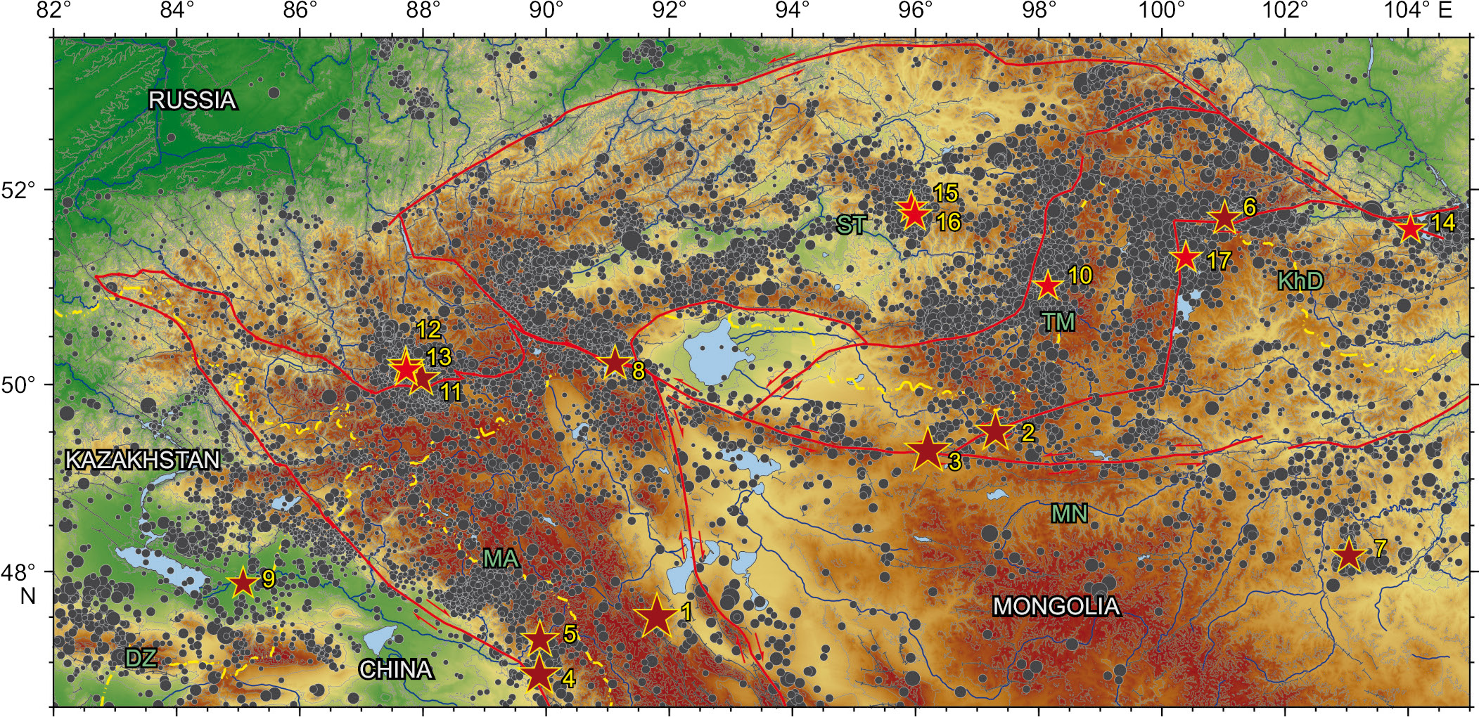
Fig. 1. Epicentral location of earthquakes in the Altai-Sayan mountain region (from the catalogue of the GS RAS, over 22000 events, 1997–2021).
Stars mark strong earthquakes: red – M≥6 earthquakes; dark red – with M≥7 earthquakes. Earthquake numbers are shown in yellow: 1 – Great Mongolian, 1761, M=8.3; 2 – Tannu-Ola, 1905, M=7.6; 3 – Bolnai, 1905, M=8.3; 4 – Fuyun, 1931, M=7.9; 5 – aftershock of the Fuyun earthquake, 1931, M=7.3; 6 – Mondy, 1950, M=7.0; 7 – Mogod, 1967, M=7.0; 8 – Ureg-Nur, 1970, M=7.0; 9 – Zaysan, 1990, M=6.8; 10 – Busingol, 1991, M=6.4; 11 – Chuya, 2003, M=7.3; 12 – aftershock of the Chuya earthquake, 2003, M=7.0; 13 – aftershock of the Chuya earthquake, 2003, M=6.9; 14 – Kultuk, 2008, M=6.4; 15 – Tuva I, 2011, M=6.6; 16 – Tuva II, 2012, M=6.8; 17 – Khubsugul, 2021, M=6.9. Letters indicate blocks [Sankov et al., 2003]: ST – Sayan-Tuva, TM – Tuva-Mongolian, KhD – Khamar Daban, MA – Mongolian Altai, DZ – Dzungar, MN – Mongolian.
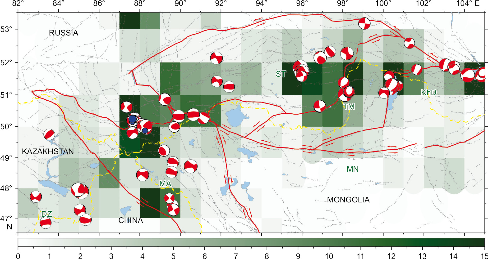
Fig. 2. Seismic moment tensors (СMT) for the earthquakes in the Altai, Sayan and adjacent areas (66 events) against the background of the annual earthquake number (more than 22000 events from 1997 to 2021 in the GS RAS catalog).
Gray lines are faults after [Bachmanov et al., 2017]. The dash-dotted line is the state border. Blue color stands for the epicenters of the earthquakes (3 events) from the GS RAS catalog for which the scalar seismic moment is known. See Fig. 1 for the block names.
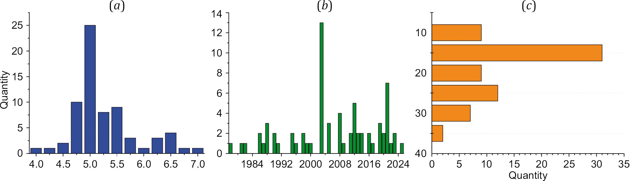
Fig. 3. Quantitative distribution of the earthquakes under consideration (69 events): (a) – by magnitude, (b) – by year, (c) – by depth.
Table 1. Model relationships between the source radius (m) and the moment magnitude; the number and range of magnitudes of the studied events; the source
No. | lg(r, [m]) | Number of events | Magnitude range МW | Source |
Theoretical | ||||
1 | 0.5MW+0.85 | Not applicable | 4.5–9.0 | [Bormann et al., 2009] |
2 | 0.5MW+0.58 | –/– | 3.0–8.0 | [Boore, 2003] |
3 | 0.4MW+1.50 | –/– | 0.12–9.20 | [Riznichenko, 1985] |
Experimental | ||||
4 | 0.2MW+1.80 | 183 | 2.5–5.5 | [Sycheva, Bogomolov, 2020] |
5 | 0.1MW+2.60 | 63 | 1.7–6.1 | [Dobrynina, 2009] |
6 | 0.22MW+2.02 | 90 | 1.6–4.2 | [Kim et al., 1989] |
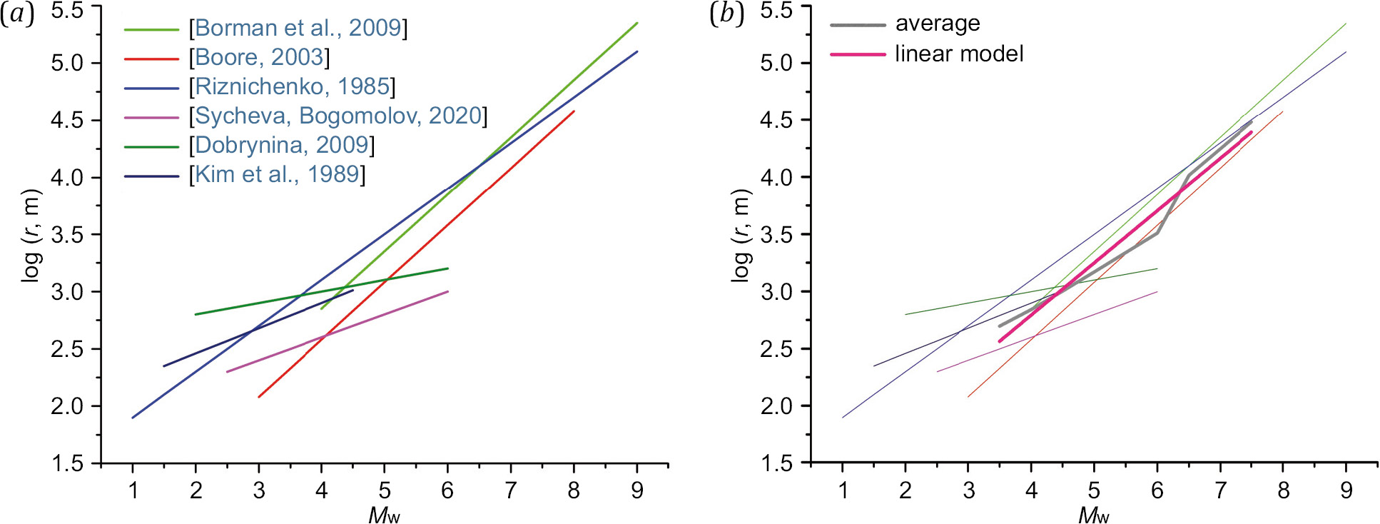
Fig. 4. Dependence of the source radius rB on the moment magnitude MW for the models under consideration (a) (Table 1), and the average value for the models and its regression (b).
The approach described in the methodology section was used to calculate the source radius, stress drops and reduced seismic energy for 65 earthquakes considered. App. 1, Table 1.1 presents the results of calculation of r and ∆σ for the Brune model. Also shown are relative values of the radiuses and stress drops; the МW=7.2 Chuya earthquake of September 27, 2003 was selected as a reference. The source radius of this earthquake in the Brune model r=~15800 m, the stress drop value ∆σ=~10 MPa.
App. 1, Table 1.1 also contains the reduced seismic energy value, which, as mentioned above, does not depend on the source model selection. The typical order of magnitude of ePR of the M=4–5 earthquakes is ~10–3, with corresponds to the results in [Dobrynina, 2009; Kocharyan, 2012]. For the earthquakes considered (MW=3.7–7.2), the average source radius is 2932 m, medium source radius – 1995 m, the average stress drop corresponds to 4.72 MPa, the medium stress drop – to 4.23 MPa, the average value of ePR=0.57⋅10–3, the medium ePR=0.51⋅10–3. Some difference between the average (mean) and medium values of the considered parameters is caused by the fact that 80 % of earthquakes vary in magnitude in the range 4.2–5.7, which is responsible for some deviations in the calculated parameters.
Fig. 5 presents the epicentral location of 69 earthquakes studied, with a circle fill color depending on the stress drop value (see the map legend that shows range ∆σ for each of the selected colors and the corresponding number of earthquakes) on the background distribution of the logarithm of seismotectonic deformation intensity [Lukk, Yunga, 1979], obtained in [Sycheva, 2023] for the Altai-Sayan mountain region. Most of the considered events fell within the areas where seismotectonic deformation intensity exceeds 10–10 year–1 (source areas of the 2003 Chuya earthquake, 2021 Khubsugul earthquake, 2011–2012 Tuva earthquakes).
The verification of stress drop and reduced seismic energy estimates, made using regressions (7) – (9), i.e. by the phenomenological method, may involve the results presented in [Zakharova et al., 2009; Chepkunas, Malyanova, 2017, 2018], where the source spectra served as a basis for determining dynamic parameters of some strong earthquakes worldwide, including 5 earthquakes in the Altai-Sayan region. The data on dynamic parameters, obtained by both methods, are available for the following earthquakes (Fig. 6):
– Chuya earthquake, September 27, 2003, MW=7.2 (No. 20 in App. 1, Table 1.1);
– aftershock of the Chuya earthquake, September 27, 2003, MW=6.4 (No. 21);
– aftershock, October 1, 2003, MW=6.6 (No. 22);
– I Tuva earthquake, December 29, 2011, MW=6.7 (No. 41);
– II Tuva earthquake, February 26, 2012, MW=6.6 (No. 42).
For these 5 earthquakes, Table 2 presents the values of some dynamic parameters determined by two methods. In the papers whose authors are the members of the staff of the Geophysical Survey RAS and referred to herein, the dynamic parameters are calculated based on the spectra of longitudinal waves obtained with STS-1 seismometers at teleseismic distances ∆≤100° from the data recorded by "Obninsk" station (OBN; 55.1146° N, 36.5674° E; h=160 m). The epicentral distance interval for the considered earthquakes varies in the range ∆=30.9–34.7°. According to [Zakharova et al., 2009; Chepkunas, Malyanova, 2017, 2018], the station spectra of the earthquakes mentioned (Table 2) were reduced to the source before determining spectral parameters Ω0 and f0.
In the analysis of Table 2, attention is drawn to the discrepancy between the scalar seismic moment value and source dimension obtained by two different methods. For M0, on the one hand, it is due to the fact that the scalar seismic moment in [Zakharova et al., 2009; Chepkunas, Malyanova, 2017, 2018] was determined by spectral parameters of longitudinal, not of transverse waves. On the other hand, the discrepancies in M0 (i.e. in energy characteristics) may be caused by the hypocentral depth error in the CMT catalog for the earthquakes considered. In publications which involved spectral parameters, the largest source dimension (source length) was determined by the Haskell’s, not by the Brune model (the model review in [Aptekman et al., 1989]), so that the difference between L and r values in Table 2 is not surprising. Dynamic parameters M0, r, L are intermediate in stress drop estimations. In view of the foregoing, when comparing values ∆σ, obtained by two methods, the question arises about a compatibility or incompatibility at least in the order of values.
According to Table 2, the calculation based on the source spectrum gave higher stress drops than that based on regressions in 4 out of 5 cases. The ratio ∆σspectrum/∆σregression does not exceed 1.6 in 3 cases and reaches 2.4 in 1 case (aftershock of the 27.09.2003 Chuya earthquake). For the Chuya earthquake, there is an inverse ratio between the values ∆σ: ∆σspectrum~0.55∆σregression. The magnitudes of 5 earthquakes considered lie in a narrow range, and the arithmetic mean ∆σ becomes important there. For two methods of stress drop calculation, the average values presented in Table 2 differ by approximately 20 %. There is the same difference in the weighted average of the values ∆σ for two methods. For the calculations from the spectra, the arithmetic mean turned out to be larger and the weighted average turned out to be smaller than for the regression-based method.
Thus, the difference in the stress drop values for two methods is less than one order of magnitude (maximum 2.4 times), which implies the possibility to use the obtained data (App. 1, Table 1.1) for ∆σ and for ePR, proportional thereto, in the Altai-Sayan region. However, for the aftershocks of the Chuya earthquake, whose magnitudes are lower and stress drops are higher than those of the main shock, the parameters are not consistent with regression. This shows that in case of aftershocks the proposed phenomenological approach may lead to errors.
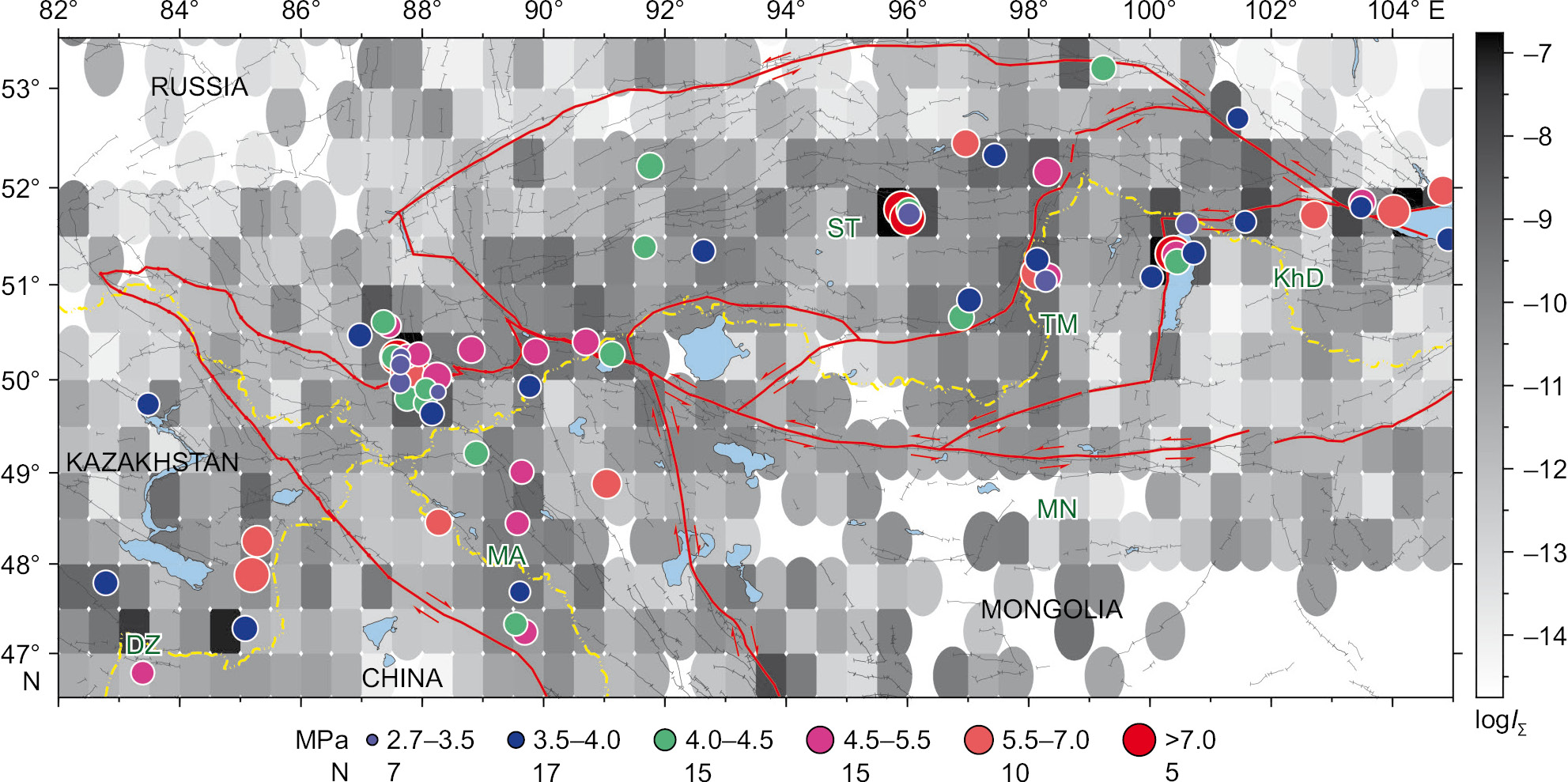
Fig. 5. Epicentral location of the earthquakes studied.
The color of the circle fill depends on the magnitude of the released stresses (see the map legend). The released stresses are calculated using the Brune earthquake source model [Brune, 1970, 1971]. For block names, see Fig. 1.
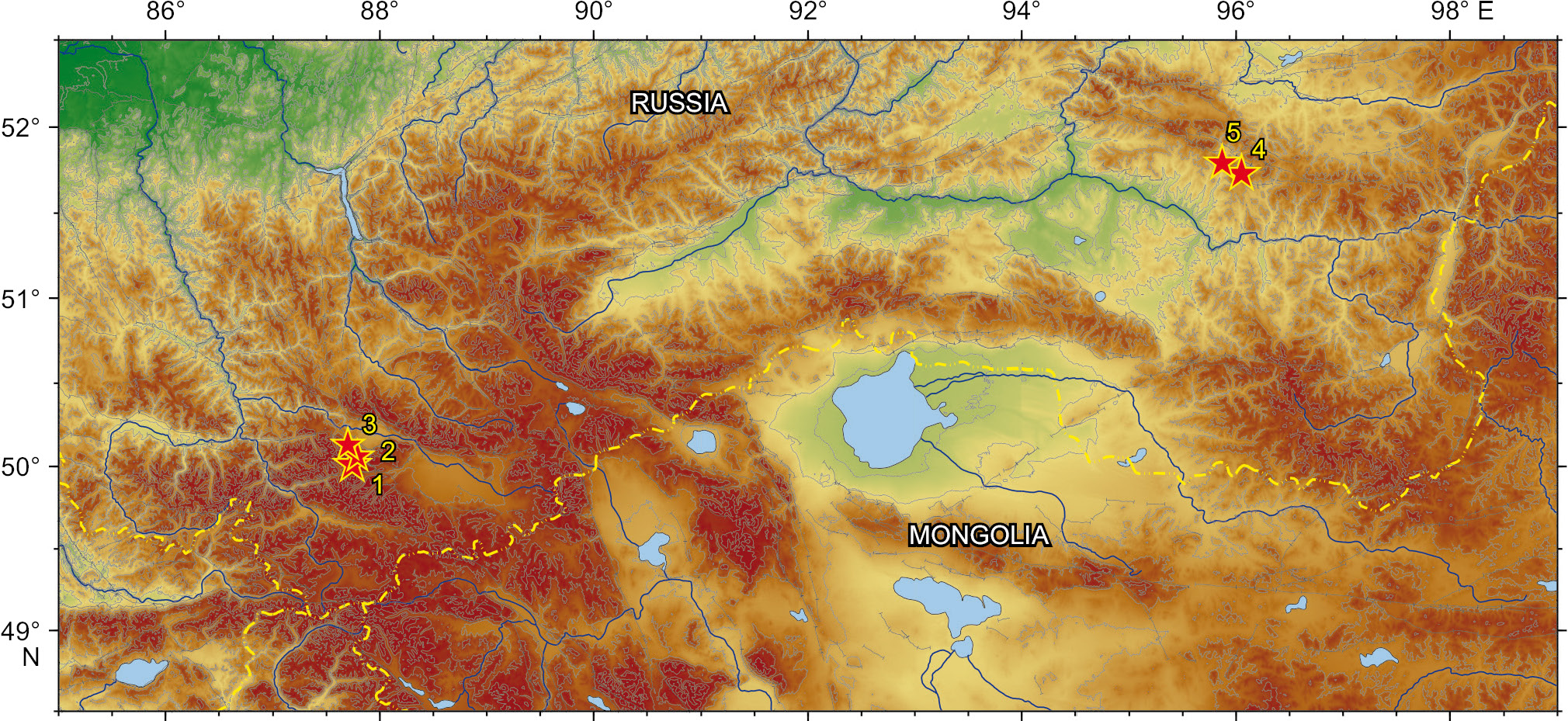
Fig. 6. Epicentral location of test earthquakes (5 events). The earthquake number corresponds to the number in Table 2.
Table 2. The values of scalar seismic moment, rupture length L, source radius and shear stress drop, according to [Zakharova et al., 2009; Chepkunas, Malyanova, 2017, 2018] and the results presented here (App. 1, Table 1.1)
No. | Date | Time | From the source spectrum | Phenomenological approach | ||||||
MW | M0·1019, N·m | L·103, m | ∆σ·105, N/m2 | MW | M0·1019, N·m | rB·103, m | ∆σ·105, N/m2 | |||
1 | September 27, 2003 | 11:33:26.5 | 6.9 | 2.2 | 24 | 56 | 7.2 | 9.38 | 15.8 | 103.1 |
2 | September 27, 2003 | 18:52:47.1 | 6.2 | 0.2 | 9 | 96 | 6.4 | 0.45 | 6.92 | 60 |
3 | October 1, 2003 | 01:03:25.0 | 6.3 | 0.4 | 9 | 192 | 6.6 | 1.13 | 8.51 | 80 |
4 | December 27, 2011 | 15:21:54.9 | 6.6 | 0.9 | 14 | 115 | 6.7 | 1.38 | 9.44 | 72 |
5 | February 26, 2012 | 06:17:18.0 | 6.8 | 1.5 | 18 | 90 | 6.6 | 1.2 | 8.5 | 84 |
Average of ∆σ·105 | 110 | Average of ∆σ·105 | 80 | |||||||
Weighted average of ∆σ·105 | 76.5 | Weighted average of ∆σ·105 | 92.6 | |||||||
The stress drop values are related to the source area, i.e. to a rather small volume of the medium. The analysis of the relationship among the stress drops, geodynamic environments and the large-scale averaged parameters of the stress-strain state of the earth’s crust requires averaging ∆σ over some event sampling. The sampling in the study region was performed by 1×1° zoning. The volumes of sources, in which the shear stress drops occur, are different for different events and represent different proportions of the volume of the medium for the study zone. Therefore, the averaging of the stress drops over sampling naturally involves introducing weighting coefficient gi, proportional to the source volume, i.e. gi~ri3, where i is an event number in the sampling. The weighted average of the stress drops <Δσ>AW will be determined by the expression:
 (10)
(10)
Since Δσiri3=7/16(M0)i, this expression can be reduced to the following calculation formula for the weighted average of the stress drops:
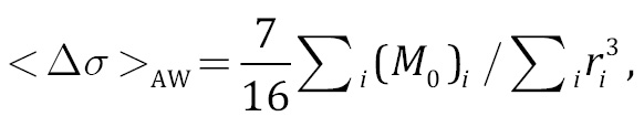 (11)
(11)
where the summation is performed over all sample events, M0i, is a scalar seismic moment of the earthquake number "i", and ri is the source radius value calculated by the Brune model.
Averaging resulted in obtaining ∆σAW for 36 cells of size 1×1°. 24 cells were contacted by 1 event, and the averaged ∆σAW corresponds to the stress drop during an earthquake. For the rest of the cells, the averaged ∆σAW depends on the number of earthquakes in a cell.
Fig. 7, a, shows the ellipse-shaped cells for which the values ∆σAW have been obtained. To visualize (to map) the calculation results, use has been made of the GMT program nearneighbor (Generic Mapping Tools, https://www.generic-mapping-tools.org/), which implements the nearest neighbor algorithm to assign the average value to every node which has one or several points within the assigned radius therefrom. This program considers a node as the center of an elliptical (circular) zone to which the calculated average applies. A cell color depends on value of the logarithmic average of the stress drops (logarithmic scale provides more contrasting delineation patterns of the cells with the minimum stress drop value). Each cell shows the number of events fell therein. Most of the events fell within the cell which coincides with the source area of the Chuya earthquake. The dark-blue cells (15 of 36) have ∆σAW ≤4 MPa, and 7 zones have ∆σAW≥6.5 MPa (source area of the Chuya earthquake ~9 MPa, Tuva earthquakes ~8 MPa, Busingol earthquake ~6.5 MPa etc.).
High stress drop falls within the northern boundaries of the Mongolian-Altai block (the Chuya earthquake area, Septmber 27, 2003, MW=7.2, and further east), northwestern and southeastern boundaries of the Tuva-Mongolian block, southeastern part of the Sayan-Tuva block; high stress drop is also typical of Jungar block area (Fig. 7, а).
Fig. 7, b, presents the logarithmic distribution of the total reduced seismic energy, calculated also for 1×1° cells. The proper value lgePR is shown for the cells contacted only by one event. It is natural that the areal distribution of lg(ΣePR) is similar to the distribution of lg∆σAW (Fig. 7, а) due to (4). Some differences (the cells south of the northern boundaries of the Mongolian-Altai block) are caused by the fact that the summation of ePR within a cell is performed irrespectively of the source volumes. Fig. 7, b, depicts zones with the maximum values of total ePR: the northern boundary of the Mongolian-Altai block, ΣePR~(0.8–6.0)⋅10–3, and the northwestern and southeastern boundaries of the Tuva-Mongolian block, ΣePR~(0.2–3.0)⋅10–3.
As a result of the application of the phenomenological approach for calculating the source radius (without plotting the source spectrum of earthquake seismograms), an assessment was made of the shear stress drops and reduced seismic energy for 69 earthquakes occurred in the Altai-Sayan mountain region. This allowed the comparison between ∆σ and ePR for different events and different zones (App. 1, Table 1.1 presents for convenience the relative values ∆σ).
To compare the stress drop value (dynamic parameter) with the Lode – Nadai coefficient distribution (kinematic parameter), the joint mapping of these parameters was carried out for the study area (Fig. 8). The considered parameters were compared within the area for which the Lode – Nadai coefficient distribution has been obtained [Sycheva, Rebetsky, 2024]. From among the events considered, 59 fell within the cells with the known values of the Lode – Nadai coefficient. The calculation was made of the number of events and of the total stress drop for the earthquakes in the areas with different deformation modes which were determined by the Lode – Nadai coefficient value. Table 3 presents some results of the quantitative analysis. In the areas of uniaxial extension (µε≤–0.6, blues in the legend), there are no events considered.
According to the data presented in Table 2, 26 (~44 %) earthquakes are located in the area of uniaxial compression deformation and uniaxial compression dominance. The total stress drop, an average with weighting factor proportional to the source volume ∆σAW, calculated by (11), was 4 MPa. The pure shear deformation area is associated with localization of 27 (~46 %) earthquakes and the stress drop ∆σAW of 8.9 MPa. In the area of the uniaxial extension dominance, there are 6 (10 %) earthquakes, and the stress drop ∆σAW was 5.6 MPa. When the kinematic characteristics of earthquakes are compared to their dynamic characteristics, it is apparent that most of the stress drops occurred in the areas with µε>0.2, which corresponds to the mode of uniaxial compression deformation and uniaxial compression dominance. The source area of the Chuya earthquake is associated with the mode of uniaxial compression dominance (Fig. 8). The stress drop during the Chuya earthquake was ~10 MPa.
Concluding the description of the distributions of reduced seismic energy and stress drops for the earthquakes in the Altai-Sayan region, we emphasize the features of the proposed phenomenological method. This method is based on the generalizations concerning the relationship between the source radius and scalar seismic moment (or moment magnitude). The phenomenological model (regression) considers a large amount of data from different publications. This does not require determination of the values of angular frequencies, which are often scattered. Nevertheless, the applicability of the phenomenological method for other seismoactive regions remains a question, which should be considered in each individual case (it is particularly important to recognize how small the proportion of aftershocks is in the sample with a known seismic moment). The proposed method for assessing stress drops and reduced seismic energy will make it possible to increase significantly the available data concerning dynamic parameters.
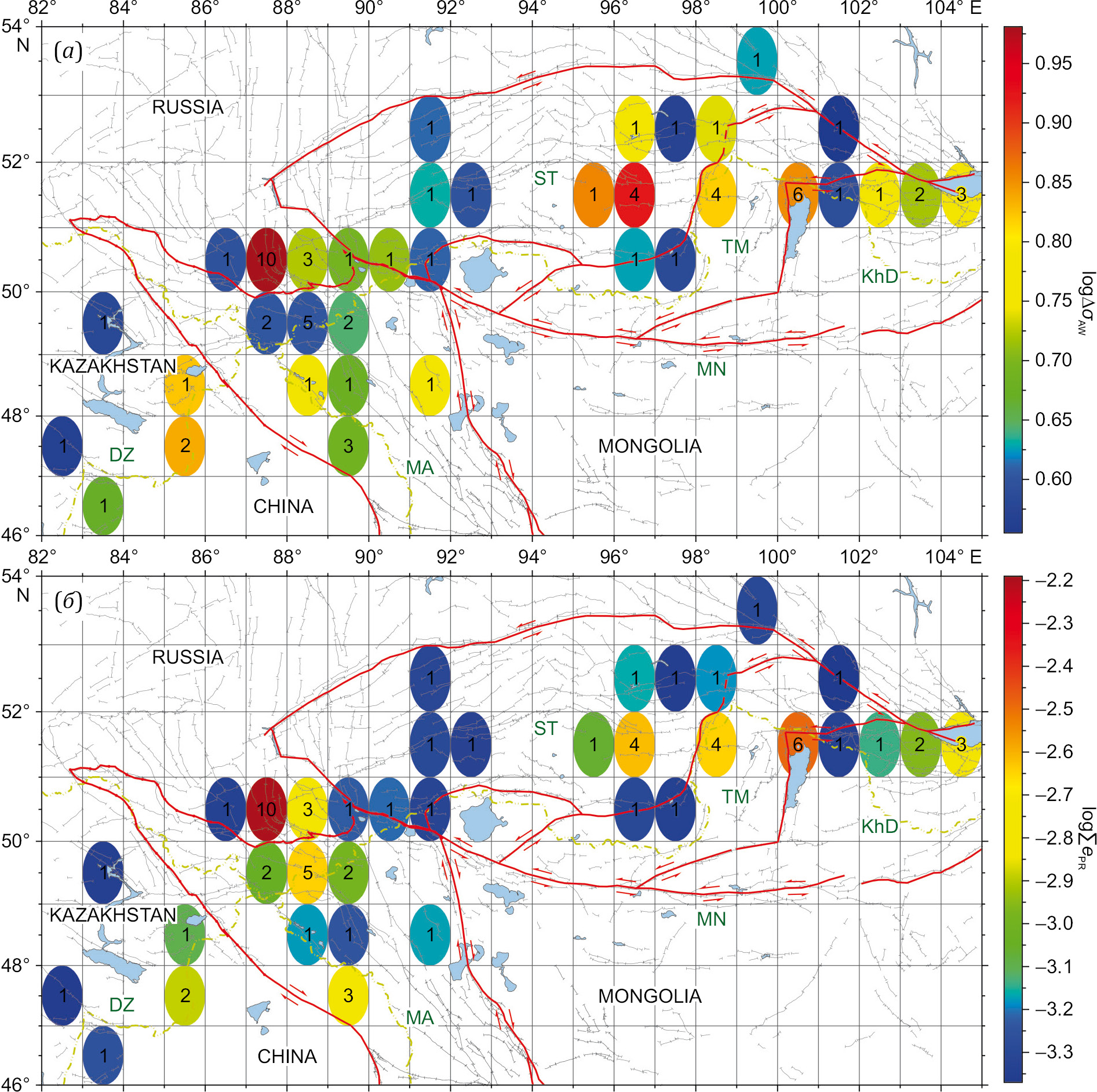
Fig. 7. Distribution of logarithm values: (a) – dropped stresses ∆σAW; (b) – total reduced seismic energy. The numbers indicate the number of events fell therein. For block names, see Fig. 1.
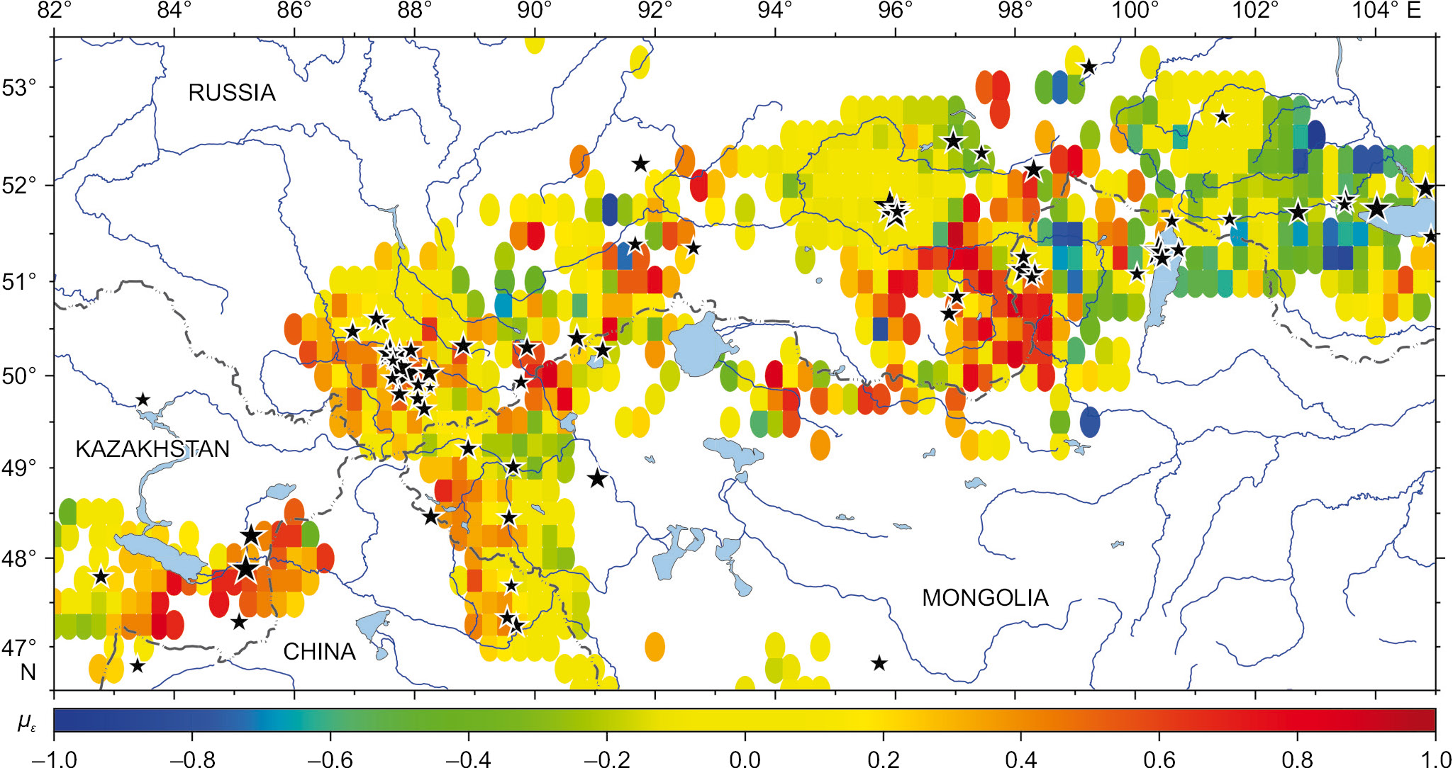
Fig. 8. Epicentral location of earthquakes on the background distribution of the Lode – Nadai coefficient, after [Sycheva, Rebetsky, 2024].
Table 3. The stress drop values ∆σ and the Lode – Nadai coefficient µε [Sycheva, Rebetsky, 2024] in zones of different defotmation modes
Factor | Deformation modes | ||||
Uniaxial compression | Uniaxial compression dominance | Pure shear | Uniaxial compression | Uniaxial extension | |
με | 0.6≤με≤1.0 | 0.2<με<0.6 | –0.2≤με≤0.2 | –0.6<με<–0.2 | –1.0≤με≤–0.6 |
∆σAW, MPa | 4.0 | 8.9 | 7.3 | 5.6 | 0 |
N | 2 | 24 | 27 | 6 | 0 |
The present paper proposes the phenomenological approach to the calculation of the source radius without plotting a source spectrum. Analysis has been made on the previously determined theoretical and empirical relationships between the source radius and the moment magnitude. Averaging of these relationships served as a basis for derivation of the expressions for calculating the shear stress drops and reduced seismic energy from the data on the scalar seismic moment or the moment magnitude. The proposed approach has been used for the earthquakes in the Altai-Sayan mountain region to increase the amount of data on the stress drops ∆σ and reduced seismic energy ePR. There is a correspondence between the regression-based estimates of stress drops for 5 test earthquakes (phenomenological approach) and the estimates previously calculated from the source spectral parameters.
Among the earthquakes that hit this area in 1978–2025, there were selected 69 events whose scalar seismic moments and moment magnitudes (MW=4.75–5.50) are listed in the CMT catalog. Regarding these events, the estimates have been made on ∆σ and ePR, and the databank has been compiled from the dynamic parameters (App. 1, Table 1.1). For mapping the areal stress drop distributions, it has been proposed to use the weighted averages ∆σ, considering the difference in source volumes of the averaged (compactly located) events. For most of the 1×1° zones, in which the stress drop averaging was performed, the values ∆σAW do not exceed 4.5 MPa, and the maximum weighted average stress drop ∆σAW is ~9 MPa. The same zones in the study area are characterized by the reduced seismic energy values ePR~0.58⋅10–3.
A comparative analysis of the kinematic and dynamic parameters of earthquakes has shown that most of the stress drops ∆σAW fell within the areas with µε>0.2, which corresponds to the mode of uniaxial compression deformation and uniaxial compression dominance.
Table 1.1. Dynamic parameters of earthquakes (69 events) in the Altai-Sayan mountain region
No. | Date | Time | φ, ° | λ, ° | H, km | MW | M0·1017 (N·m) | rB, m | ∆σ, MPa | ePR·10–3 | rB norm | ∆σ norm |
1 | 03.08.1978 | 06:07:41.10 | 52.45 | 96.96 | 10.0 | 5.6 | 3.60 | 3020 | 5.72 | 0.69 | 0.19 | 0.56 |
2 | 16.08.1981 | 17:54:18.10 | 50.84 | 97.02 | 15.0 | 5.2 | 0.70 | 1995 | 3.86 | 0.46 | 0.13 | 0.37 |
3 | 03.08.1982 | 04:50:29.60 | 49.01 | 89.64 | 10.0 | 5.1 | 0.62 | 1799 | 4.67 | 0.56 | 0.11 | 0.45 |
4 | 24.04.1986 | 00:22:17.20 | 47.33 | 89.54 | 33.0 | 5.0 | 0.43 | 1622 | 4.44 | 0.53 | 0.10 | 0.43 |
5 | 04.11.1986 | 16:19:20.20 | 50.32 | 88.81 | 15.0 | 5.5 | 2.44 | 2723 | 5.29 | 0.63 | 0.17 | 0.51 |
6 | 18.09.1987 | 21:58:39.90 | 47.24 | 89.69 | 15.0 | 5.3 | 1.28 | 2213 | 5.17 | 0.62 | 0.14 | 0.50 |
7 | 30.06.1988 | 15:25:13.90 | 50.27 | 91.13 | 15.0 | 5.3 | 1.01 | 2213 | 4.08 | 0.49 | 0.14 | 0.40 |
8 | 23.07.1988 | 07:38:15.00 | 48.88 | 91.04 | 18.0 | 5.9 | 8.99 | 4121 | 5.62 | 0.67 | 0.26 | 0.55 |
9 | 14.06.1990 | 12:47:32.60 | 47.88 | 85.19 | 36.0 | 6.6 | 97.30 | 8511 | 6.90 | 0.83 | 0.54 | 0.67 |
10 | 03.08.1990 | 09:15:12.50 | 48.25 | 85.28 | 32.0 | 6.1 | 19.80 | 5070 | 6.65 | 0.80 | 0.32 | 0.65 |
11 | 27.12.1991 | 09:09:45.80 | 51.12 | 98.14 | 15.0 | 6.3 | 37.50 | 6237 | 6.76 | 0.81 | 0.39 | 0.66 |
12 | 22.06.1995 | 01:01:23.80 | 50.30 | 89.87 | 15.0 | 5.4 | 1.67 | 2455 | 4.94 | 0.59 | 0.15 | 0.48 |
13 | 29.06.1995 | 23:02:33.10 | 51.72 | 102.71 | 15.0 | 5.7 | 5.20 | 3350 | 6.05 | 0.73 | 0.21 | 0.59 |
14 | 12.03.1996 | 18:43:48.30 | 48.46 | 88.27 | 17.0 | 5.5 | 2.56 | 2723 | 5.55 | 0.67 | 0.17 | 0.54 |
15 | 12.07.1998 | 07:16:21.20 | 47.79 | 82.78 | 35.4 | 5.2 | 0.67 | 1995 | 3.68 | 0.44 | 0.13 | 0.36 |
16 | 21.11.1998 | 16:59:54.10 | 49.21 | 88.89 | 15.0 | 5.2 | 0.74 | 1995 | 4.08 | 0.49 | 0.13 | 0.40 |
17 | 25.02.1999 | 18:58:39.00 | 51.97 | 104.83 | 21.0 | 5.9 | 8.91 | 4121 | 5.57 | 0.67 | 0.26 | 0.54 |
18 | 31.05.2000 | 16:28:07.80 | 51.47 | 104.92 | 15.0 | 5.0 | 0.38 | 1622 | 3.91 | 0.47 | 0.10 | 0.38 |
19 | 07.05.2003 | 02:58:02.01 | 48.45 | 89.57 | 33.0 | 5.1 | 0.64 | 1799 | 4.78 | 0.57 | 0.11 | 0.46 |
20 | 27.09.2003 | 11:33:36.25 | 50.02 | 87.86 | 15.0 | 7.2 | 938.00 | 15849 | 10.31 | 1.24 | 1.00 | 1.00 |
21 | 27.09.2003 | 18:52:52.93 | 50.09 | 87.75 | 15.0 | 6.4 | 45.20 | 6918 | 5.97 | 0.72 | 0.44 | 0.58 |
22 | 01.10.2003 | 01:03:29.98 | 50.24 | 87.59 | 15.0 | 6.6 | 113.00 | 8511 | 8.02 | 0.96 | 0.54 | 0.78 |
23 | 04.10.2003 | 14:23:29.00 | 49.87 | 88.26 | 0 | 3.7 | 0.00 | 422 | 2.61 | 0.31 | 0.03 | 0.25 |
24 | 05.10.2003 | 16:21:13.00 | 50.16 | 87.64 | 0 | 4.4 | 0.05 | 871 | 3.32 | 0.40 | 0.05 | 0.32 |
25 | 06.10.2003 | 18:30:17.40 | 50.24 | 87.65 | 0 | 4.2 | 0.03 | 708 | 3.10 | 0.37 | 0.04 | 0.30 |
26 | 09.10.2003 | 16:06:03.16 | 49.75 | 88.05 | 15.0 | 5.0 | 0.41 | 1622 | 4.24 | 0.51 | 0.10 | 0.41 |
27 | 13.10.2003 | 05:26:42.32 | 50.25 | 87.75 | 15.0 | 5.1 | 0.60 | 1799 | 4.51 | 0.54 | 0.11 | 0.44 |
28 | 17.10.2003 | 05:30:25.90 | 50.27 | 87.94 | 15.0 | 5.1 | 0.61 | 1799 | 4.55 | 0.55 | 0.11 | 0.44 |
29 | 23.10.2003 | 00:25:48.46 | 49.64 | 88.16 | 15.0 | 5.1 | 0.48 | 1799 | 3.64 | 0.44 | 0.11 | 0.35 |
30 | 11.11.2003 | 22:42:35.69 | 50.47 | 86.97 | 15.0 | 5.1 | 0.53 | 1799 | 3.95 | 0.47 | 0.11 | 0.38 |
31 | 17.11.2003 | 01:35:52.31 | 50.24 | 87.53 | 15.0 | 5.2 | 0.75 | 1995 | 4.15 | 0.50 | 0.13 | 0.40 |
32 | 15.02.2005 | 12:41:45.28 | 47.69 | 89.61 | 13.2 | 4.6 | 0.10 | 1072 | 3.70 | 0.44 | 0.07 | 0.36 |
33 | 27.04.2005 | 07:36:15.28 | 51.09 | 98.33 | 12.0 | 5.3 | 1.28 | 2213 | 5.17 | 0.62 | 0.14 | 0.50 |
34 | 22.08.2005 | 08:31:25.94 | 49.97 | 87.63 | 27.4 | 4.7 | 0.13 | 1189 | 3.31 | 0.40 | 0.07 | 0.32 |
35 | 19.01.2008 | 07:32:31.71 | 51.26 | 98.14 | 12.0 | 5.1 | 0.49 | 1799 | 3.69 | 0.44 | 0.11 | 0.36 |
36 | 29.01.2008 | 20:02:30.72 | 49.74 | 83.48 | 34.8 | 4.9 | 0.27 | 1462 | 3.82 | 0.46 | 0.09 | 0.37 |
37 | 16.08.2008 | 04:01:11.67 | 52.16 | 98.31 | 28.2 | 5.7 | 4.70 | 3350 | 5.47 | 0.66 | 0.21 | 0.53 |
38 | 27.08.2008 | 01:35:38.61 | 51.76 | 104.02 | 23.5 | 6.3 | 34.10 | 6237 | 6.15 | 0.74 | 0.39 | 0.60 |
39 | 04.08.2009 | 16:20:43.23 | 50.66 | 96.89 | 30.4 | 5.3 | 1.05 | 2213 | 4.24 | 0.51 | 0.14 | 0.41 |
40 | 10.02.2011 | 05:35:17.82 | 52.22 | 91.76 | 26.3 | 5.5 | 1.89 | 2723 | 4.10 | 0.49 | 0.17 | 0.40 |
41 | 27.12.2011 | 15:22:03.84 | 51.78 | 95.91 | 19.5 | 6.7 | 138.00 | 9441 | 7.18 | 0.86 | 0.60 | 0.70 |
42 | 26.02.2012 | 06:17:24.34 | 51.69 | 96.00 | 20.5 | 6.6 | 119.00 | 8511 | 8.44 | 1.01 | 0.54 | 0.82 |
43 | 26.02.2012 | 11:59:05.84 | 51.74 | 96.03 | 17.6 | 5.1 | 0.54 | 1799 | 4.02 | 0.48 | 0.11 | 0.39 |
44 | 06.06.2012 | 14:04:17.47 | 51.77 | 96.02 | 28.0 | 5.2 | 0.78 | 1995 | 4.31 | 0.52 | 0.13 | 0.42 |
45 | 27.07.2012 | 03:58:13.43 | 51.73 | 96.03 | 17.9 | 4.9 | 0.25 | 1462 | 3.46 | 0.41 | 0.09 | 0.34 |
46 | 30.07.2012 | 22:30:43.73 | 50.61 | 87.36 | 25.9 | 5.1 | 0.57 | 1799 | 4.29 | 0.51 | 0.11 | 0.42 |
47 | 24.01.2013 | 07:35:37.30 | 49.80 | 87.75 | 19.6 | 5.2 | 0.76 | 1995 | 4.16 | 0.50 | 0.13 | 0.40 |
48 | 30.04.2013 | 01:03:33.34 | 51.35 | 92.64 | 12.0 | 5.0 | 0.39 | 1622 | 3.98 | 0.48 | 0.10 | 0.39 |
49 | 01.11.2014 | 00:52:01.56 | 52.70 | 101.45 | 29.8 | 4.8 | 0.19 | 1318 | 3.59 | 0.43 | 0.08 | 0.35 |
50 | 05.12.2014 | 18:04:22.68 | 51.33 | 100.72 | 22.8 | 5.0 | 0.35 | 1622 | 3.61 | 0.43 | 0.10 | 0.35 |
51 | 13.07.2016 | 06:45:48.63 | 49.93 | 89.77 | 31.2 | 4.9 | 0.28 | 1462 | 3.93 | 0.47 | 0.09 | 0.38 |
52 | 20.09.2016 | 07:18:14.06 | 49.90 | 88.06 | 18.7 | 4.8 | 0.23 | 1318 | 4.35 | 0.52 | 0.08 | 0.42 |
53 | 04.04.2017 | 15:07:31.43 | 47.28 | 85.08 | 32.6 | 5.3 | 0.96 | 2213 | 3.89 | 0.47 | 0.14 | 0.38 |
54 | 01.02.2019 | 21:54:43.19 | 46.78 | 83.39 | 26.0 | 5.0 | 0.46 | 1622 | 4.67 | 0.56 | 0.10 | 0.45 |
55 | 29.03.2019 | 23:22:06.97 | 51.65 | 101.57 | 21.9 | 4.8 | 0.20 | 1318 | 3.90 | 0.47 | 0.08 | 0.38 |
56 | 13.09.2019 | 04:08:04.81 | 50.57 | 87.45 | 20.7 | 5.1 | 0.63 | 1799 | 4.70 | 0.56 | 0.11 | 0.46 |
57 | 21.09.2020 | 18:05:00.13 | 51.85 | 103.50 | 25.9 | 5.5 | 2.49 | 2723 | 5.40 | 0.65 | 0.17 | 0.52 |
58 | 21.09.2020 | 18:19:58.18 | 51.80 | 103.48 | 18.5 | 4.8 | 0.20 | 1318 | 3.74 | 0.45 | 0.08 | 0.36 |
59 | 11.01.2021 | 21:33:07.45 | 51.32 | 100.39 | 13.9 | 6.8 | 190.00 | 10471 | 7.24 | 0.87 | 0.66 | 0.70 |
60 | 13.01.2021 | 11:10:11.81 | 51.63 | 100.61 | 12.0 | 4.8 | 0.18 | 1318 | 3.48 | 0.42 | 0.08 | 0.34 |
61 | 21.02.2021 | 01:37:08.94 | 52.33 | 97.44 | 27.4 | 5.0 | 0.36 | 1622 | 3.73 | 0.45 | 0.10 | 0.36 |
62 | 31.03.2021 | 00:01:29.29 | 51.24 | 100.45 | 24.9 | 5.3 | 1.02 | 2213 | 4.12 | 0.49 | 0.14 | 0.40 |
63 | 03.05.2021 | 08:46:41.95 | 51.31 | 100.43 | 27.5 | 5.7 | 4.21 | 3350 | 4.90 | 0.59 | 0.21 | 0.48 |
64 | 06.09.2021 | 07:47:21.91 | 53.20 | 99.23 | 24.9 | 5.3 | 1.05 | 2213 | 4.24 | 0.51 | 0.14 | 0.41 |
65 | 22.10.2021 | 23:03:04.95 | 51.39 | 91.67 | 29.8 | 5.0 | 0.42 | 1622 | 4.28 | 0.51 | 0.10 | 0.42 |
66 | 29.07.2022 | 13:01:14.18 | 50.40 | 90.70 | 13.0 | 5.5 | 2.37 | 2723 | 5.14 | 0.62 | 0.17 | 0.50 |
67 | 14.01.2023 | 07:39:34.60 | 51.08 | 100.03 | 19.9 | 4.9 | 0.26 | 1462 | 3.67 | 0.44 | 0.09 | 0.36 |
68 | 04.03.2023 | 01:18:25.17 | 51.04 | 98.28 | 19.7 | 4.8 | 0.17 | 1318 | 3.27 | 0.39 | 0.08 | 0.32 |
69 | 15.02.2025 | 01:48:13.11 | 50.03 | 88.24 | 26.0 | 5.8 | 6.20 | 3715 | 5.29 | 0.63 | 0.23 | 0.51 |
1. Abdrakhmatov K.Ye., Aldazhanov S.A., Hager B.H., Hamburger M.W., Herring T.A., Kalabaev K.B., Makarov V.I., Molnar P. et al., 1996. Relatively Recent Construction of the Tien Shan Inferred from GPS Measurements of Present-Day Crustal Deformation Rates. Nature 384, 450–453. https://doi.org/10.1038/384450a0.
2. Aivazian S.A., 2001. Applied Statistics. Essentials of Econometrics. Vol. 2. Essentials of Econometrics. Textbook. Unity-Dana, Moscow, 432 p. (in Russian)
3. Aivazian S.A., Mkhitarian V.S., 2001. Applied Statistics. Essentials of Econometrics. Vol. 1. Theory and Applied Statistics. Textbook. Unity-Dana, Moscow, 656 p. (in Russian)
4. Aptekman Zh.Ya., Belavina Yu.F., Zakharova A.I., Zobin V.M., Kogan S.Ya., Korchagina O.A., Moskvina A.G., Polikarpova L.A., Chepkunas L.S., 1989. P-wave Spectra in the Context of Determining the Dynamic Source Parameters of Earthquakes. Station to Source Spectrum Transition and Calculation of Dynamic Source Parameters. Journal of Volcanology and Seismology 2, 66–79 (in Russian)
5. Bachmanov D.M., Kozhurin A.I., Trifonov V.G., 2017. The Active Faults of Eurasia Database. Geodynamics & Tectonophysics 8 (4), 711–736 (in Russian) https://doi.org/10.5800/GT-2017-8-4-0314.
6. Boore D., 2003. Simulation of Ground Motion Using the Stochastic Method. Pure and Applied Geophysics 160 (3–4), 635–676. https://doi.org/10.1007/PL00012553.
7. Bormann P., Liu R., Xu Z., Ren K., Zhang L., Wendt S., 2009. First Application of the New IASPEI Teleseismic Magnitude Standards to Data of the China National Seismographic Network. Bulletin of the Seismological Society of America 99 (3), 1868–1891. https://doi.org/10.1785/0120080010.
8. Brune J.N., 1970. Tectonic Stress and the Spectra of Seismic Shear Waves from Earthquakes. Journal of Geophysical Research 75 (26), 4997–5009. https://doi.org/10.1029/JB075i026p04997.
9. Brune J.N., 1971. Correction [to "Tectonic Stress and the Spectra of Seismic Shear Waves from Earthquakes"]. Journal of Geophysical Research 76 (20), 5002. https://doi.org/10.1029/JB076i020p05002.
10. Chepkunas L.S., Malyanova L.S., 2017. Source Parameters of Strong Earthquakes. Earthquakes of the Northern Eurasia. Iss. 20 (2011). GS RAS, Obninsk, p. 277–281 (in Russian)
11. Chepkunas L.S., Malyanova L.S., 2018. Source Parameters of Strong Earthquakes. Earthquakes of the Northern Eurasia. Iss. 21 (2012). GS RAS, Obninsk, p. 280–285 (in Russian)
12. Chinnery V.A., 1961. The Deformation of the Ground Around Surface Faults. Bulletin of the Seismological Society of America 51 (3), 355–3725. https://doi.org/10.1785/BSSA0510030355.
13. Chinnery V.A., 1969. Earthquake Magnitude and Source Parameters. Bulletin of the Seismological Society of America 59 (5), 1969–1982. https://doi.org/10.1785/BSSA0590051969.
14. Dobrynina A.A., 2009. Source Parameters of the Earthquakes of the Baikal Rift System. Izvestiya, Physics of the Solid Earth 45 (12), 1093–1109. https://doi.org/10.1134/S1069351309120064.
15. Emanov A.F., Emanov A.A., Chechel’nitskii V.V., Shevkunova E.V., Radziminovich Ya.B., Fateev A.V., Kobeleva E.A., Gladyshev E.A., Arapov V.V., Artemova A.I., Podkorytova V.G., 2022. The Khuvsgul Earthquake of January 12, 2021 (MW=6.7, ML=6.9) and Early Aftershocks. Izvestiya, Physics of the Solid Earth 58, 59–73. https://doi.org/10.1134/S1069351322010025.
16. Emanov A.F., Emanov A.A., Chechelnitsky V.V., Shevkunova E.V., Kobeleva E.A., Fateev A.V., 2023. The Block Structure and the Strongest Earthquakes of the Junction Area Between the Altai-Sayan Mountain Region and the Baikal Rift Zone. In: Problems of Complex Geophysical Monitoring of Seismoactive Regions. Proceedings of the 9th Scientific-Technical Conference with an International Participation (September 24–30, 2023). Kamchatka Branch of the GS RAS, Petropavlovsk-Kamchatsky, p. 139–142 (in Russian)
17. Emanov A.F., Emanov A.A., Fateev A.V., Soloviev V.M., Shevkunova E.V., Gladyshev E.A., Antonov I.A., Korabelshchikov D.G. et al., 2021. Seismological Studies in the Altai-Sayan Mountain Region. Russian Journal of Seismology 3 (2), 20–51 (in Russian) https://doi.org/10.35540/2686-7907.2021.2.02.
18. Emanov A.F., Emanov A.A., Leskova E.V., 2010. Seismic Activation in the Busingol-Belinsky Fault Zone. Physical Mesomechanics 13 (S1), 72–77 (in Russian)
19. Emanov A.F., Emanov A.A., Leskova E.V., Seleznev V.S., Fateev A.V., 2014a. The Tuva Earthquakes of December 27, 2011, ML=6.7, and February 26, 2012, ML=6.8, and Their Aftershocks. Doklady Earth Sciences 456 (1), 594–597. https://doi.org/10.1134/S1028334X14050249.
20. Emanov A.F., Leskova E.V., Emanov A.A., Radziminovich Ya.B., Gileva N.A., Artemova A.I., 2014b. The August 16, 2008, Belin-Bii-Khem Earthquake with КР=15, МW=5.7, I0=7 (the Tuva Republic). Earthquakes of the Northern Eurasia. Iss. 17 (2008). GS RAS, Obninsk, p. 378–385 (in Russian)
21. Kanamori H., 1977. The Energy Release in Great Earthquakes. Journal of Geophysical Research 82 (20), 2981–2987. https://doi.org/10.1029/JB082i020p02981.
22. Kaneko Y., Shearer P.M., 2014. Seismic Source Spectra and Estimated Stress Drop Derived from Cohesive-Zone Models of Circular Subshear Rupture. Geophysical Journal International 197 (2), 1002–1015. https://doi.org/10.1093/gji/ggu030.
23. Kim W.-Y., Wahlström R., Uski M., 1989. Regional Spectral Scaling Relations of Source Parameters for Earthquakes in the Baltic Shield. Tectonophysics 166 (1–3), 151–161. https://doi.org/10.1016/0040-1951(89)90210-2.
24. Kocharyan G.G., 2012. On Radiation Efficiency of Earthquakes (an Example of Geomechanical Interpretation of the Results of Seismological Observations). Dynamic Processes in Geospheres 3, 36–47 (in Russian)
25. Kocharyan G.G., 2014. Scale Effect in Seismotectonics. Geodynamics & Tectonophysics 5 (2), 353–385 (in Russian) https://doi.org/10.5800/GT-2014-5-2-0133.
26. Kocharyan G.G., 2016. Geomechanics of Faults. GEOS, Moscow, 424 p. (in Russian)
27. Kostrov B.V., 1975. Mechanics of Tectonic Earthquake Source. Nauka, Moscow, 176 p. (in Russian)
28. Kuchai O.A., 2012. Specific Features of Fields of Stresses Associated with Aftershock Processes in the Altai-Sayan Mountainous Region. Geodynamics & Tectonophysics 3 (1), 59–68 (in Russian) https://doi.org/10.5800/GT-2012-3-1-0062.
29. Larson K.M., Bürgmann R., Bilham R., Freymueller J.T., 1999. Kinematics of the India-Eurasia Collision Zone from GPS Measurements. Journal of Geophysical Research: Solid Earth 104 (B1), 1077–1093. https://doi.org/10.1029/1998JB900043.
30. Logachev N.A. (Ed.), 1993. Seismotectonics and Seismicity of Lake Khövsgöl Region. Nauka, Novosibirsk, 184 p. (in Russian)
31. Lukk A.A., Yunga S.L., 1979. Seismotectonic Deformation of the Garm Region. Bulletin of the USSR Academy of Sciences. Physics of the Earth 10, 24–43 (in Russian)
32. Madariaga R., 2011. Earthquake Scaling Laws. In: R. Meyers (Ed.), Extreme Environmental Events: Complexity in Forecasting and Early Warning. Springer, New York, p. 364–383. https://doi.org/10.1007/978-1-4419-7695-6_22.
33. Misharina L.A., Melnikova V.I., Baljinnyam I., 1983. South-Western Boundary of the Baikal Rift Zone from the Data on Earthquake Focal Mechanisms. Volcanology and Seismology 2, 74–83 (in Russian)
34. Riznichenko Yu.V., 1985. Problems of Seismology. Nauka, Moscow, 408 p. (in Russian)
35. Sankov V.A., Levi K.G., Lukhnev A.V., Miroshnichenko A.I., Parfeevets A.V., Radziminovich N.A., Melnikova V.I., Deverchere J. et al., 2002. Recent Geodynamics of the Mongol-Siberian Mobile Belt from the Geological-Structural and Instrumental Data. In: Tectonics and Geophysics of the Lithosphere. Proceedings of the XXXV Tectonic Meeting (January 1 – December 31, 2002). Vol. 2. GEOS, Moscow, p. 170–174 (in Russian)
36. Sankov V.A., Lukhnev A.V., Miroshnichenko A.I., Levi K.G., Ashurkov S.V., Bashkuev Yu.B., Dembelov M.G., Calais E. et al., 2003. Present-Day Movements of the Earth’s Crust in the Mongol-Siberian Region Inferred from GPS Geodetic Data. Doklady Earth Sciences 393 (8), 1082–1085.
37. Scholz C.H., 2002. The Mechanics of Earthquakes and Faulting. Cambridge University Press, Cambridge, 496 p. https://doi.org/10.1017/CBO9780511818516.
38. Sycheva N.A., 2023. Study of Seismotectonic Deformations of the Earth’s Crust in the Altai-Sayan Mountain Region. Part I. Geosystems of Transition Zones 7 (3), 223–242 (in Russian) https://doi.org/10.30730/gtrz.2023.7.3.223-242.
39. Sycheva N.A., Bogomolov L.M., 2016. Patterns of Stress Drop in Earthquakes of the Northern Tien Shan. Russian Geology and Geophysics 57 (11), 1635–1645. https://doi.org/10.1016/j.rgg.2016.10.009.
40. Sycheva N.A., Bogomolov L.M., 2020. On the Stress Drop in North Eurasia Earthquakes Source Versus Specific Seismic Energy. Geosystems of Transition Zones 4 (4), 393–446. https://doi.org/10.30730/gtrz.2020.4.4.393-416.417-446.
41. Sycheva N.A., Bogomolov L.M., Kuzikov S.I., 2020. Computational Technologies in Seismological Research (on the Example of KNET, Northern Tian Shan). IMGG FEB RAS, Yuzhno-Sakhalinsk, 358 p. (in Russian) https://doi.org/10.30730/978-5-6040621-6-6.2020-2.
42. Sycheva N.A., Rebetsky Yu.L., 2024. Comparing the STDand MCA-Based Estimates of the Crustal Deformation in the Altai-Sayan Mountain Region. In: Tectonophysics and Challenges in Earth Sciences. Proceedings of the Sixth Tectonophysical Conference to the 300th Anniversary of the Russian Academy of Sciences (October 7–12, 2024). IPE RAS, Moscow, p. 329–336 (in Russian)
43. Sycheva N.A., Sychev V.N., 2022. Some Characteristics of Seismicity in the Altai and Sayan Mountains. In: Problems of Geocosmos – 2022. Proceedings of the XIV School-Conference with an International Participation (October 3–7, 2022). Skifia-Print, Saint Petersburg, p. 84–92 (in Russian)
44. Vakov A.V., 1988. Relationships Between Earthquake Magnitude and Source Dimensions at Different Types of Fault Movements. Collection of Gidroproekt Scientific Papers. Iss. 130. Energoizdat, Moscow, p. 55–69 (in Russian)
45. Zakharova A.I., Chepkunas L.S., Malyanova L.S., 2009. Source Parameters of Strong Earthquakes. Earthquakes of the Northern Eurasia. Iss. 12 (2003). GS RAS, Obninsk, p. 255–260 (in Russian)
46. Zavyalov A.D., Zotov O.D., 2021. A New Way to Determine the Characteristic Size of the Source Zone. Journal of Volcanology and Seismology 15 (1), 19–25. https://doi.org/10.1134/S0742046321010139.
10-1 Bolshaya Gruzinskaya St, Moscow 123242
1B Nauki St, Yuzhno-Sakhalinsk 693022
Sycheva N.A., Bogomolov L.M. DISTRIBUTION OF REDUCED SEISMIC ENERGY AND STRESS DROP IN THE ALTAI-SAYAN SEISMOACTIVE REGION. Geodynamics & Tectonophysics. 2025;16(4):0835. https://doi.org/10.5800/GT-2025-16-4-0835. EDN: VWPTKO


Editor-in-Chief
Sklyarov E.V.664033, Irkutsk, Lermontova St., 128,
IEC SB RAS Institute of the Earth's crust
E-mail.: gt@crust.irk.ru
tel.: 8 3952 425422
Processing of personal data


