


Contents
Scroll to:
https://doi.org/10.5800/GT-2024-15-2-0751
EDN: AAFHCI
Scroll to:
The Gebel EL-Zeit area in the southwestern Gulf of Suez, Egypt, is an area with a significant hydrocarbon potential in sedimentary basins, so that the three-stage inversion method was proposed for the Bouguer anomalies observed therein. Salt diapirs obscured the deep structure of the main central El-Zeit basin; hence, this method was implemented to overcome challenges in 3D seismic modeling. Our study included direct and inverse parameterization sequences that involved analyzing the inputs and outputs within trial-and-error initiations and inverse estimations to assess whether and how much the constraining parameters used in the calculations could achieve the intended aim. Data reduction, filtering, optimization, and constraint assumptions were used to determine the minimal set of density model parameters needed to set limits on the acceptable range of density contrasts that are required to study the basement depths, swells, troughs, faulting/folding and intra-sedimentary structures, and for direct modeling aimed at creating a simple model to save time. The thirteen constrained wells with a total depth ranging from shallow to deep were not involved in direct modeling but provided quality control over the graphical display of the inverse results for the entire study area. Moreover, many parameter constraints were inverted to regulate the way the calculated data are related to the model’s solution that allowed us to determine which inversion trial provided the best parameterization sequence and, therefore, yielded the most appropriate solution for the depth-density model which is approximating reality with a minimal computation error in the study area.
Hassan A., Farag K., Aref A., Piskarev A.L. METHODS FOR 3D INVERSION OF GRAVITY DATA IN INDENTIFYING TECTONIC FACTORS CONTROLLING HYDROCARBON ACCUMULATIONS IN THE EL ZEIT BASIN AREA, SOUTHWESTERN GULF OF SUEZ, EGYPT. Geodynamics & Tectonophysics. 2024;15(2):0751. https://doi.org/10.5800/GT-2024-15-2-0751. EDN: AAFHCI
The field sources, sedimentary basins and their anomalous densities therein cause the observed gravity anomalies – a nonlinear inverse problem for calculating the basement’s uneven surface morphology. Many inversion models fit gravity observations due to the non-uniqueness of gravity anomaly modelling [Crossley et al., 2013]. An efficient Fast Fourier Transform (FFT)-derived direct modelling approach is based on an iterative use of the sediment-basement rock density contrast and the mean basement depth to solve this interpretation problem [Fan et al., 2021; Jessell et al., 2014]. The slab formula (g=2πγΔρt) predicts sediment thickness for each gravity datum using the gravitational constant (γ), density contrast (Δρ), and slab thickness (t). The slab formula modifies the starting model when the observed-predicted data misfit is below threshold. Many researchers modified the nonlinearity of this technique [Silva et al., 2014] by changing the iteration step size, using a density-depth function instead of a fixed density, and improving the fitting function.
L. Cordell and N. Henderson separated the modelled and expected gravity anomalies from the previous iteration to alter Bott’s iterative process step size [Pham et al., 2018]. J.B.C. Silva suggested speeding convergence through separating the residual (the difference between observed and modelled gravity) by an arbitrary, relatively large inherent value and verifying the model when the L2 norm of the residual vector is less than the previous iteration [Silva et al., 2014]. Geology and void fraction affect sediment density. Fitting is needed for the direct computation of the model iteration field [Silva et al., 2014]. Fourier-domain approaches are faster than space-domain approaches. For example, analytical formulas for prismatic bodies with parabolic or cubic polynomial density contrast functions [Mallesh et al., 2019; Wu, 2019], formulas for polyhedral bodies with a linear density contrast function [Ren et al., 2017], and algorithms for modelling vertical variation of density contrast with depth require an exponential or cubic polynomial fitting function [Wu, 2016, 2018; Wu, Lin, 2017].
R. Jachens and G. Phelps used Bott’s technique to calculate and reduce the basement density-induced gravitational influence [Preston et al., 2020; Stolk et al., 2013]. The basement gravity is mapped using Nevada isostatic residual gravity anomalies to reflect basement density changes [Preston et al., 2020]. C. Martins rebuilt a model without penalizing fast morphological changes and using the total variation function corresponding to the L1 norm of the discrete derivative in basement depth inversion [Dadak, 2017]. X. Feng and J. Sun devised a nonlinear inverse technique that minimizes an objective function using a composite regularizing function to adjust model smoothness in the study area [Maag, Li, 2018; Feng et al., 2018]. Edge analysis or first-approximation models can identify unique gravity anomalies. Basement depth measurements are controlled geologically by ITRESC methods, which estimate a constant density contrast or density depth function. We intend to compare between the ITRESC results in the southwestern Gulf of Suez and in the El Zeit basin.
The Gulf of Suez was formed by the late Oligocene and early Miocene African and Arabian tectonic plate movements [Abuzied et al., 2020; Makled et al., 2020]. Low-angle listric normal faulting and dyke injection created the eastward-trending half grabens along the rift fault blocks [Bendaoud et al., 2019]. By the middle to late Miocene, the crustal weakness caused active subsidence moving the rift axis eastward into the asymmetric axial grabens. Esh El-Mallaha, a structural block in the southern Gulf of Suez intra-rift system, faulted and grew during the Pliocene to Pleistocene/Holocene [Van Dijk et al., 2019]. Tectonic faults and deep sedimentary sequences generated a half-graben in the Pre-Cretaceous central lowlands into the present-day Gemsa-El Zeit Bay basin [Faris et al., 2015; Radwan et al., 2021; Youssef et al., 2016].
The oldest to youngest Gemsa-El Zeit Bay basin lithostratigraphic units are Nubian Sandstone, the El Mallaha formation, the pre-rift upper Cretaceous Raha formation in the eastern and southern parts, the pre-rift lower Eocene Thebes formation, syn-rift lower Miocene Nukhul formation, syn-rift lower/middle Miocene Rudeis and Kareem strata, and Sabkhas and salt marshes [Almalki, Mahmud, 2018; Elgammal, Orabi, 2019; Said, 2017; Hadada et al., 2021; Van Dijk et al., 2019]. As seen in Fig. 1, a, Gebel El Zeit and Esh El-Mallaha show complex basement outcrops east and west of the Gemsa-El Zeit Bay, with a large sedimentary basin in the center.
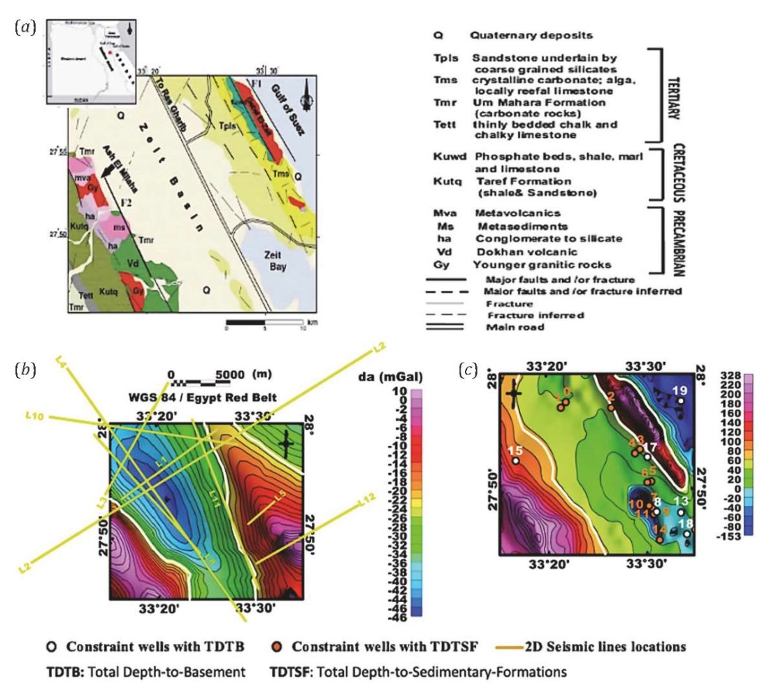
Fig. 1. The study area.
(a) – surface geologic map (after [Youssef et al., 2016]);
(b) – Bouguer gravity anomaly contour map;
(c) – topographic contour map.
Рис. 1. Район исследований.
(a) – геологическая карта (по [Youssef et al., 2016]);
(b) – карта гравитационной аномалии Буге;
(c) – топографическая карта.
The Gemsa-El-Zeit Bay basin needs further investigations because of the lack of the drilled stratigraphic-control wells and poor seismic interpretations. Gravimetry enhances deep potential-field survey investigations, and the accessible stratigraphic-control wells in the El-Zeit basinal area, listed in Table 1, can indirectly help to constrain and build the earth model during inversion trials.
Table 1. A priori information on the accessible and accessible actual total depths
to the basement of constrained wells
Табл. 1. Предварительная информация о доступной и общей глубине фундамента,
полученная с помощью буровых скважин
|
Well symbol |
Well Name |
Total Depth (m) |
Company |
Status |
|
1st / wells with T.D rock unit [basement] and geologic age/ Pre-Cambrian |
||||
|
W8 |
C9A–1 |
2577 |
Conco |
Abandoned tested oil and gas |
|
W13 |
QQ89–11 |
1129 |
DEOCO |
Abandoned |
|
W15 |
Wadi Dib #1 |
3769 |
CHEV EGY |
Abandoned |
|
W17 |
Gazwarina # 1 |
2162 |
Marathon |
Suspended oil |
|
W18 |
QQ89–3 |
2908 |
SUCO |
Abandoned |
|
W19 |
ERDMA–2 |
4051 |
Published [Aboud et al., 2005] |
|
|
2st / wells with T.D rock unit [Nubia Sandstone (Nu)] and geologic age / Carboniferous-Jurassic |
||||
|
W2 |
Kabrite west-1 |
1272 |
Petrozeit |
Abandoned oil stain |
|
W3 |
Gazwarina-2 |
1272 |
Marathon |
Abandoned oil shows |
|
W5 |
Gebel El Zeit-west-1 |
1966 |
Deminex |
Abandoned |
|
W6 |
Gebel El Zeit-west-2 |
2195 |
Deminex |
Abandoned |
|
W11 |
East Ras Gemsa-4 |
2542 |
Gupco |
Abandoned gas shows |
|
3st / wells with T.D rock unit [Matulla formation(Ma)] and geologic age / Upper Cretaceous |
||||
|
W9 |
Khalig El Zeit-1 |
2509 |
Devon |
Abandoned |
|
W10 |
East Ras Gemsa-2 |
2538 |
Gupco |
Abandoned |
|
W16 |
Zeit Bay 1 |
4452 |
CHEV EGY |
Abandoned |
|
4st / wells with T.D rock unit [Nukhul formation(Nuk)] and geologic age / Lower Miocene |
||||
|
W0 |
Gebel El Zeit-2 |
3743 |
GPC |
Abandoned |
|
5st / wells with T.D rock unit [Rudies formation (Ru)] and geologic age / Lower Miocene |
||||
|
W1 |
Ramadan-1 |
3760 |
GPC |
Abandoned oil and gas shows |
|
W4 |
Gazwarina-3 |
951 |
Marathon |
Abandoned |
|
W7 |
C9A-3 |
2122 |
Conoco |
Abandoned |
|
W14 |
C9B-1 |
3183 |
Conoco |
Abandoned |
Note. This information is used for the quality control of the inverse basement depth model results produced by the proposed inversion scheme for the study area. Sources: Ministry of Petroleum and Mineral Resources (www.petroleum.gov.eg/), Carto (https://carto.com/) and IRIS21 (http://icep.or.jp/english.html) databases.
Примечание. Эта информация используется для контроля качества результатов обратной модели глубины фундамента, полученных с помощью предлагаемой схемы инверсии для исследуемого района. Источники: Министерство нефти и минеральных ресурсов Египта (www.petroleum.gov.eg/), базы данных Carto (https://carto.com/) и IRIS21 (http://icep.or.jp/english.html).
GPC, AMOCO, GeoFisica, and Philips Petroleum have surveyed Egypt and the Gulf of Suez since 1964. The Bureau Gravimetric International (BGI) authorized the General Petroleum Company of Egypt’s (GPC) ten-year (1974–1984) gravity map of Egypt, utilizing a national base net and international company surveys. This investigation used a Lacoste and Worden gravimeter with a resolution of 0.01 mGal. The survey covered the NE-SW striking area of 32×28 km². As shown in Fig. 1, b, three intermediate-amplitude NW-SE anomalies are long-wavelength. Gravity lows between extended highs are predominant. Western gravity highs are doublets, which suggest that local transfer faults are crossing the Gebel Esh El-Mallaha at right angles. As seen in Fig. 1, c, the study area is mountainous, from 2.5 m high in the center plains to 450.0 m high in the marginal uplands.
The Gebel El Zeit study region is depicted in Fig. 2, which shows the stratigraphic succession of the southern Gulf of Suez and the correlation between the lithological column in three places [Afifi et al., 2016].
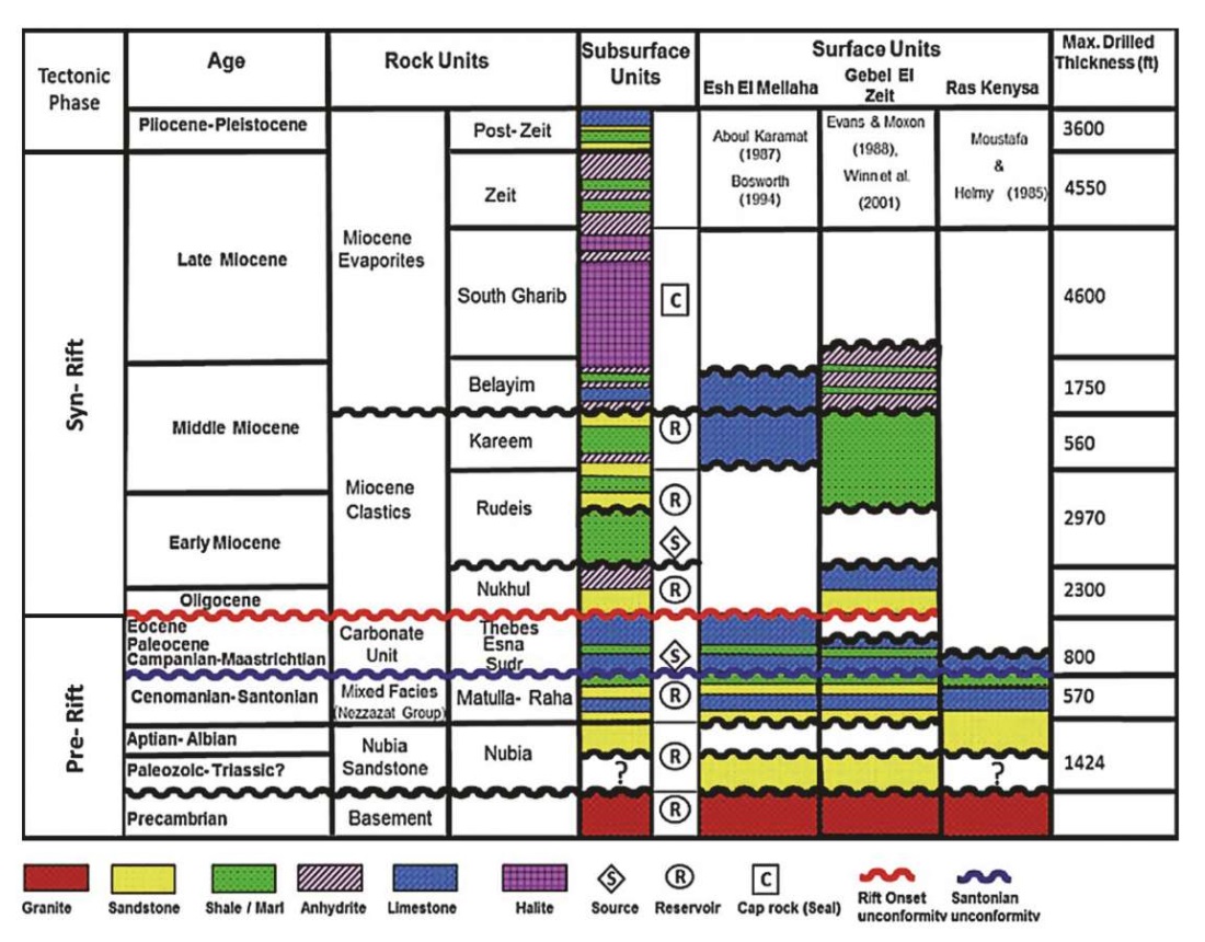
Fig. 2. Stratigraphic succession of the southern Gulf of Suez
with depiction of the correlation between the lithological column in three areas,
including the study area of Gebel El Zeit (after [Afifi et al., 2016]).
Рис. 2. Стратиграфическая последовательность для южной части Суэцкого залива
с изображением корреляции между литологической колонкой в трех областях,
включая исследуемый район Гебель-эль-Зейт (по [Afifi et al., 2016]).
General outline. Inverting Bouguer anomalies to characterize the Gebel El-Zeit basin geological features was done using the Oldenburg and other inversion methods [Oldenburg, 1974; Florio, 2018, 2020; Li, Oldenburg, 1998], incorporated within the proposed three-stage inversion scheme. In order to develop this scheme, we used the most popular extension for subroutine sequential 3D spectral layered-earth inversion modeling (GM-SYS 3D modeling) in Oasis Montaj (Geosoft Inc., Toronto, ON, Canada). The schematic stages involved hypothetical scenarios and six optimization strategies to produce optimal model solutions, three for direct modeling and three for inverse modeling. Putting indirect constraints on the inversion outcomes within the data analysis and matching the 3D inverse modeling results with the study-area subsurface geological stratigraphy, structures and stratigraphical-control wells accurately modeled the targets. In addition, the scheme involved simple direct modeling to reduce time. Fig. 3 depicts the parameterization flowchart for the proposed schematic direct and inverse modeling processes and their three stages. Table 2 provide an exhaustive list of the parameterization abbreviations used in our study.
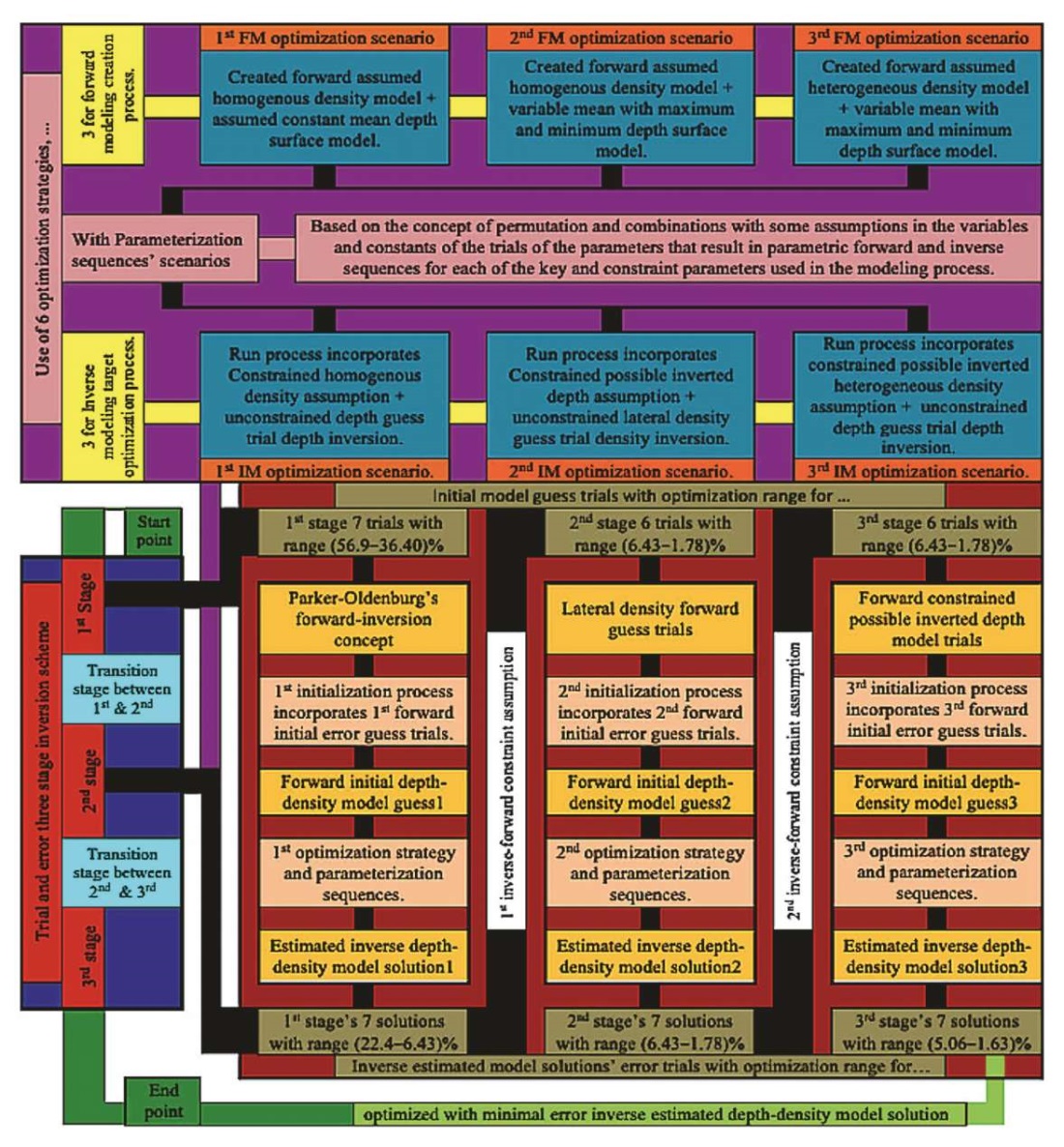
Fig. 3. The schematic depiction of the proposed inversion scheme shows three stages
of forward and inverse modeling optimization scenarios
with transitional assumptions between stages regulating the optimization process.
Рис. 3. Предложенная схема инверсии
для трех этапов оптимизации сценариев прямого и обратного моделирования
с допущениями перехода между этапами, регулирующими процесс оптимизации.
Schematic stages of inversion. The first stage involves the implementation of three optimization strategies: the first one for direct depth modeling based on the unconstrained initial direct constant mean depth surface within the 3D depth model guess trials; the second for direct density modeling that includes the initial direct density constraint assumptions of the 3D homogenous two-layered density model guess trials; and the third for depth inverse modeling estimates that combines the first two for inverting the most appropriate solution for the Oldenburg inverse model.
At the second stage, there were implemented three further optimization strategies: the first one for direct depth modeling that involves direct-constrained variable depth surfaces in 3D depth model guess trials with different depth calculation errors; the second for direct density modeling that provides a homogeneous two-layered density model by constraining the density contrast guess trials of the initial 3D constant mean density contrast interface; and the third for density inverse modeling estimates that combines the first two for inverting possible solutions of the basement complex lateral density distribution.
At the third and final stage, there are proposed three optimization strategies: the first one for the direct depth modeling that involves an unconstrained version of the second-stage direct variable depth constraint assumptions derived from the trials of inverted 3D possible depth models with varying depth calculation errors, the second for the direct density modeling that includes the constrained version of the second-stage 3D inverted lateral density contrast assuming possible solutions which yielded the third-stage depth optimality; and the third for depth inverse modeling estimates which combines the first two and in which these density-contrast constraint versions were used to evaluate the optimality of the hypothesized basement complex density and basement-sedimentary density contrast model solutions, thus providing the most appropriate solution for the minimally errored basement depth model.
Optimization and constraint assumptions were used to evaluate our three-stage inversion solution. In addition, quality control and assurance tests were done on the entire study area and in specific places using graphical schematics to figure out which inversion trial produced the optimal parameterization sequence that provided the optimal depth-density model therein.
The three-stage parameterization procedure encompasses initiating and estimating processes aimed at optimizing the key parameters of depth, density, and density contrast in the model. These parameters are illustrated in Figs 4, 6, showcasing optimization sequences inside graphs A–C and G–N. During the inversion run, the procedure incorporates constraint parameters such as the lower high-cut (LHC) and upper high-cut (UHC) filter limits, DC shift, regional offset, and convergence limit. These constraint parameters are depicted in Fig. 5, showcasing the optimization sequences represented in graphs D–F. The features with an inclined square along the X-axis in each of the graphs, A to F, highlight the optimal number of initial guesses and inverse-estimate error trials for each stage. The first stage encompasses optimization sequences of 1 to 7 trials, subsequently followed by the phase consisting of 8 to 13 trials and, finally, by the third phase involving 9 to 19 trials. See Table 2 for compilation of abbreviations.
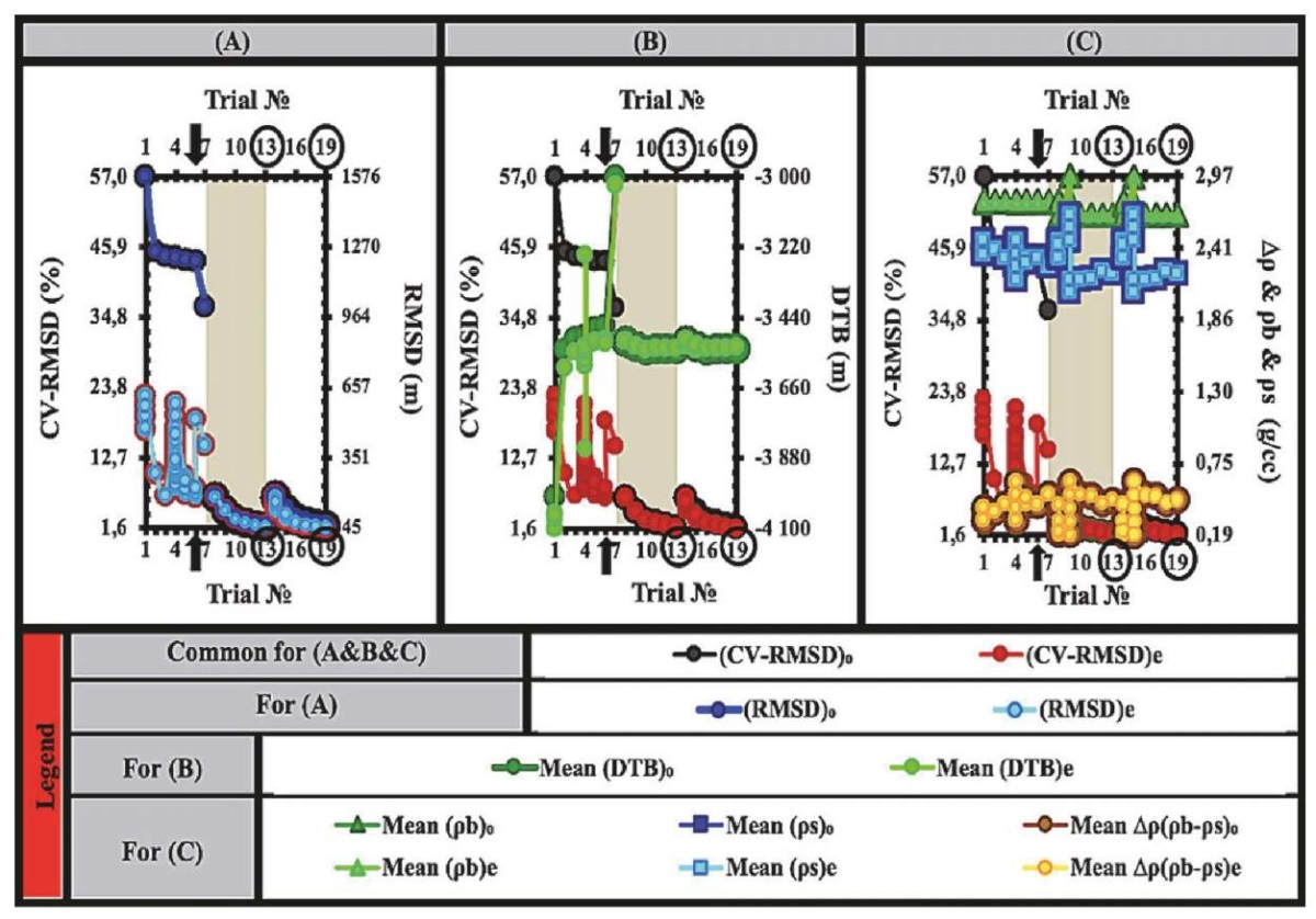
Fig. 4. A three-stage parameterization procedure. Graphs A–C (see explanation in the text).
Рис. 4. Трехэтапная процедура параметризации. Графики А–С (объяснение в тексте).
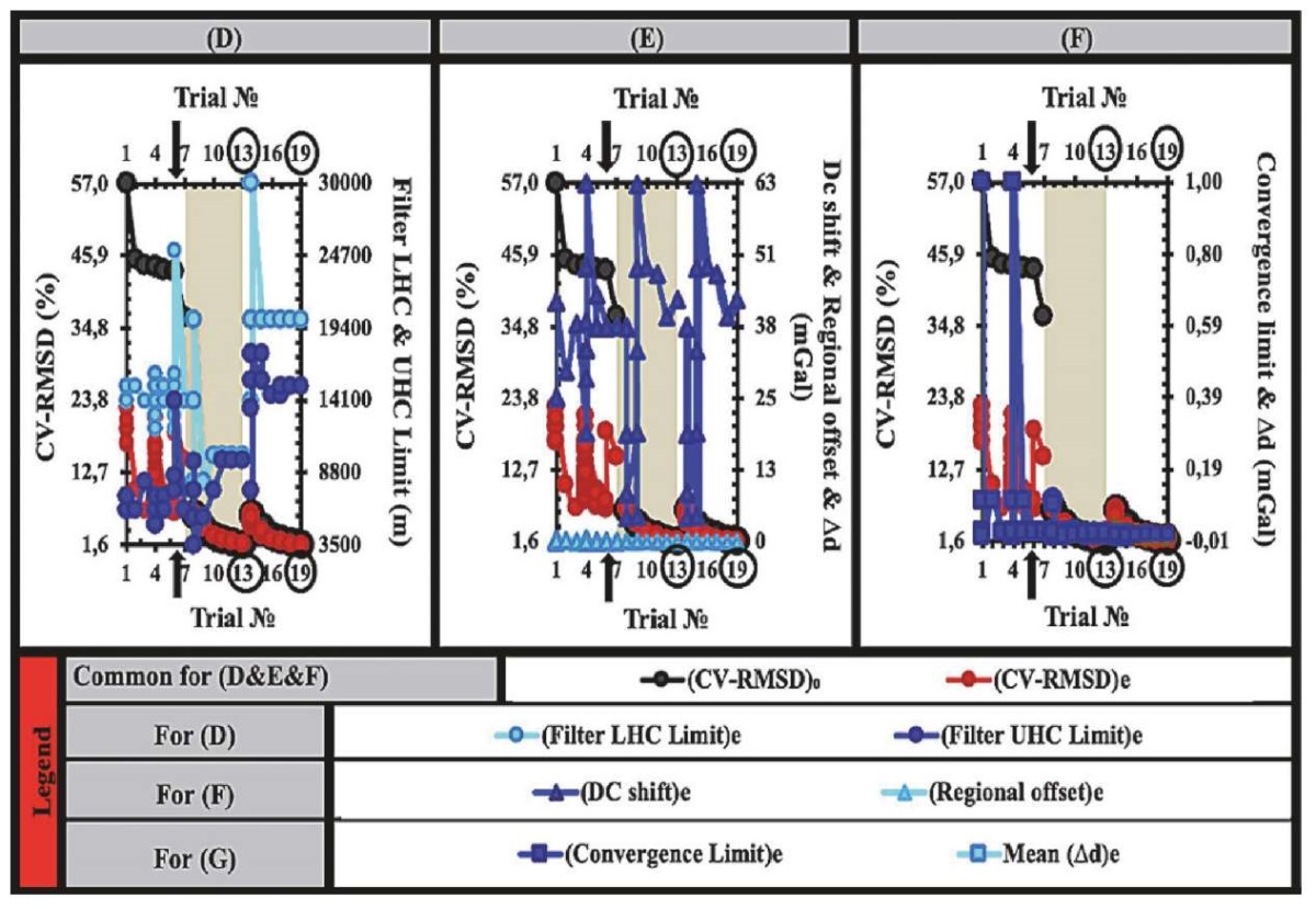
Fig. 5. A three-stage parameterization procedure. Graphs D–F (see explanation in the text).
Рис. 5. Трехэтапная процедура параметризации. Графики D–F (объяснение в тексте).
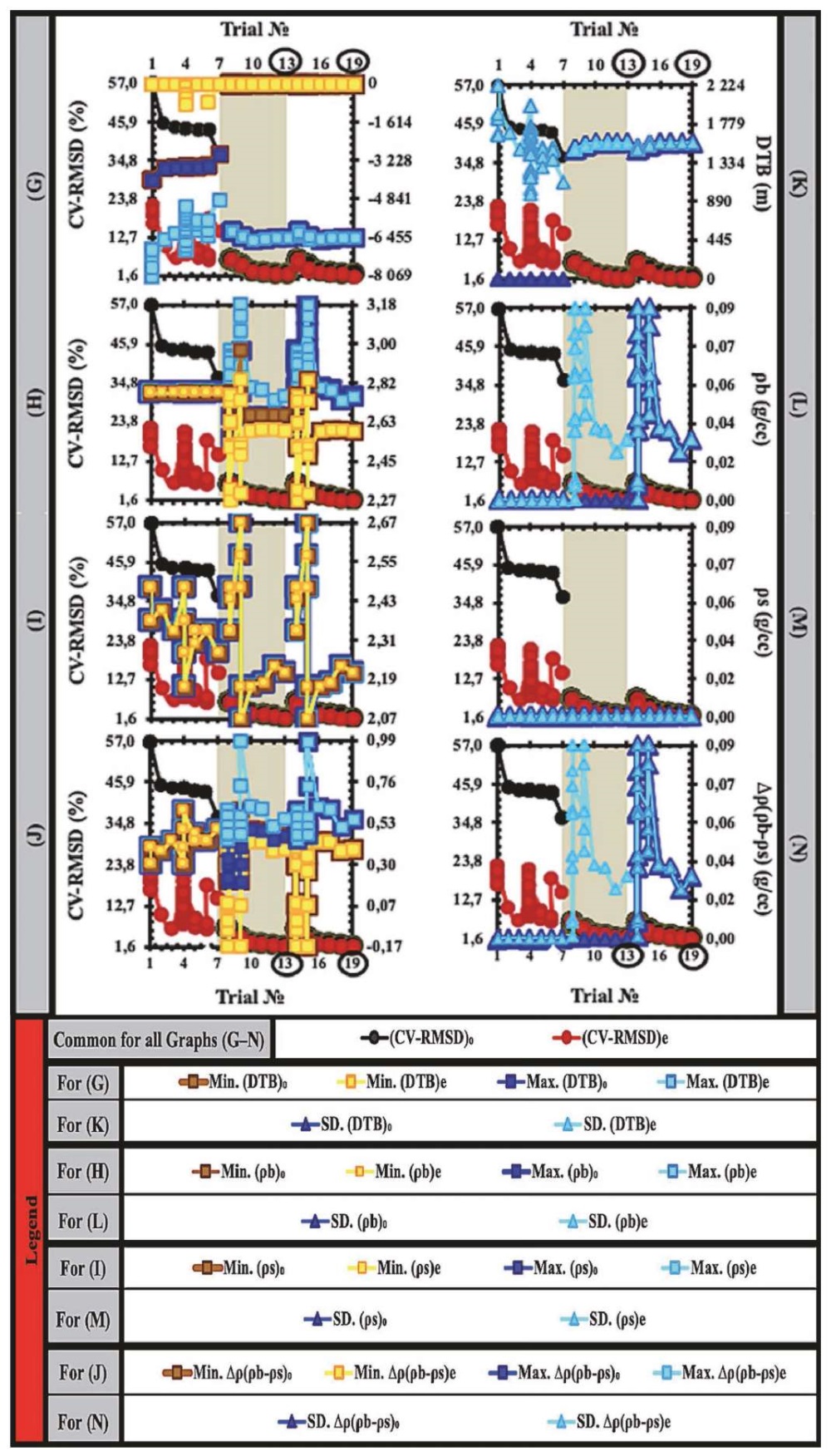
Fig. 6. A three-stage parameterization procedure. Graphs G–N (see explanation in the text).
Рис. 6. Трехэтапная процедура параметризации. Графики G–N (объяснение в тексте).
The graphical representation in Fig. 4 effectively depicts the model errors associated with the inversion scheme. The continuation of this representation can be seen in Fig. 7, where the optimal initial guess for the first stage and the inverse-estimate maps for the third stage are depicted. These maps are a part of the three-stage scheme, including three separate 3D models. The construction of these models involves parameterizations of three initial approximations that maximize the recovery of inversely estimated solutions with minimal estimation error. Fig. 7 displays the initial Oldenburg optimal guesses of the first trial and the inverse-estimate optimal recovery of the nineteenth trial in our scheme. These trials are highlighted by inclined squares along the X-axis of Fig. 4, A, which correspond to the initial assumptions and inverse modeling of the schematic first-stage ideal starting basement depth error-guess constraint. The figure visually represents the initial basement depth (Fig. 7, A), the direct assumption of homogenous density in the basement complex (Fig. 7, B), and the initial guess of the basement-sediment density contrast interface (Fig. 7, C).
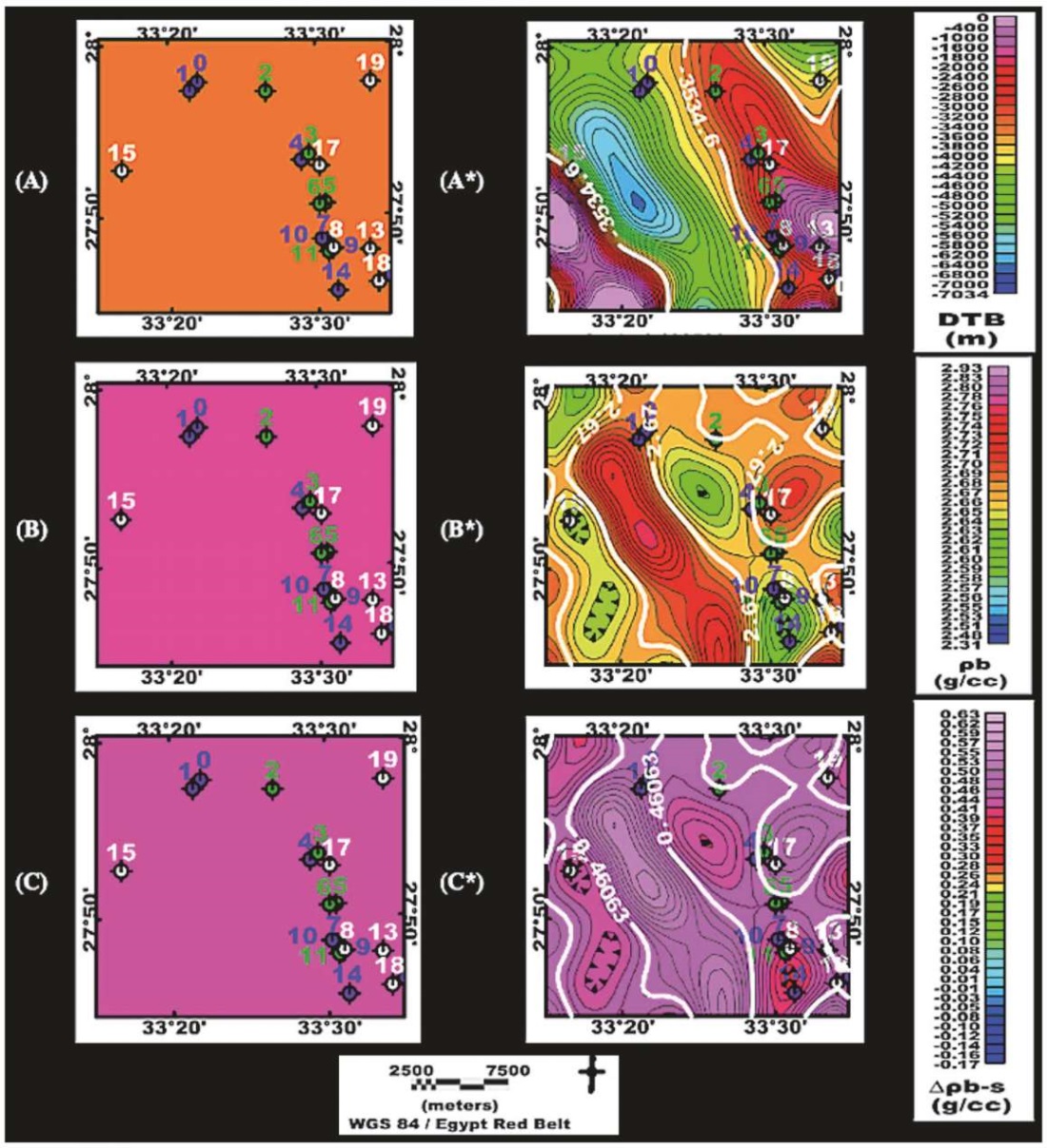
Fig. 7. Estimated 2D maps showing the first-stage optimal initial guesses
and final third-stage optimal solutions for 3D depth,
density, and density contrast in the proposed three-stage inversion scheme.
Рис. 7. Расчетные 2D-карты,
показывающие оптимальные начальные предположения первого этапа
и окончательные решения третьего этапа для 3D-моделирования глубины,
плотности и контраста плотности в предложенной трехэтапной схеме инверсии.
Furthermore, Fig. 7 also shows that the optimization sequences shown in graphs B-N, which are continued in Fig. 4, 5 and 6, provided the optimality of the model with only a 1.63 % error in the estimates of the models solutions at the nineteenth trial of the scheme (Fig. 8). This optimality is represented by the third-stage optimal inverse estimates of basement depth (see Fig. 7, A*), lateral density distribution in the basement complex (see Fig. 7, B*), and the basement-sedimentary density contrast interface (see Fig. 7, C*). Fig. 9 showing that a mean misfit of 0.00451 mGal is most appropriate to demonstrate a relationship between the observed and calculated Bouguer anomalies, as well as optimal model depth, density, and density contrast solutions shown in Fig. 7. This study presents empirical evidence substantiating the claim that the optimal solution achieved at the third stage outperforms the solutions found in the first two stages. The definitions of acronyms are provided in Table 2.
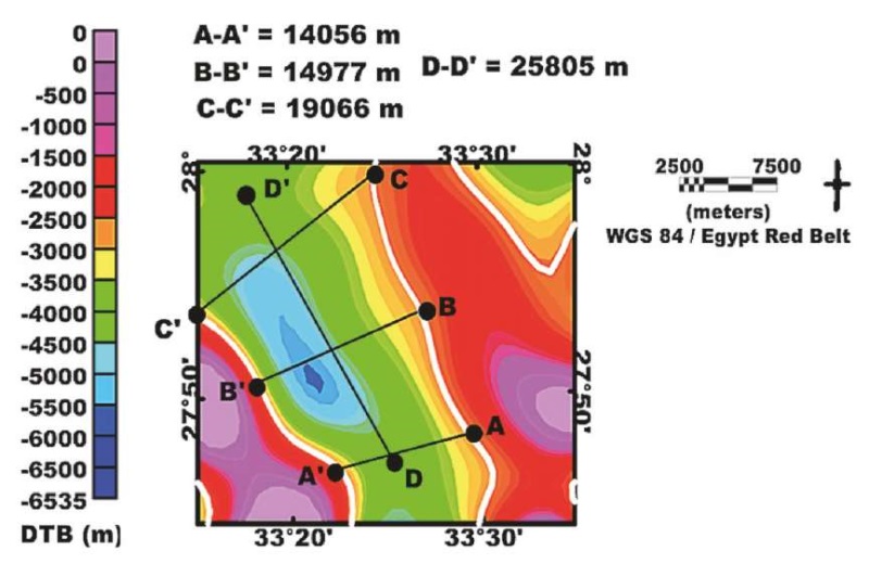
Fig. 8. 1.63 % of roughly precise dimension measurements for the El-Zeit basin
refer to the most appropriate mean depth of the white contour line
drawn on the third stage optimal-inverse basement depth map of the proposed inversion scheme.
Рис. 8. 1.63 % приблизительно точных измерений для бассейна Эль-Зейт
относятся к наиболее подходящей средней глубине белой линии,
нанесенной на карту глубин фундамента третьего этапа предлагаемой схемы инверсии.
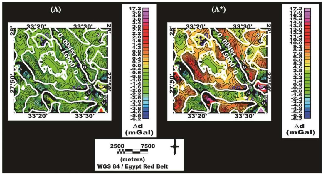
Fig. 9. Linear 2D maps, as optimal data misfit results for the proposed inversion scheme.
Рис. 9. Линейные 2D-карты как оптимальные результаты искажения данных
для предложенной схемы инверсии.
Table 2. Abbreviations and classification of the parameters
utilized in the proposed inversion scheme
Таблица 2. Сокращения и классификация параметров,
используемых в предлагаемой схеме инверсии
|
Type |
Parameter |
Parameterization meaning |
|
Root-mean-square and coefficient of variance evaluation parameters |
RMSDDTB0 |
The Root-Mean-Square Deviation of the Directly Initiated Depth-to-Basement |
|
RMSDDTBe |
The Root-Mean-Square Deviation of the Inversely Estimated Depth-to-Basement |
|
|
CV–RMSDDTB0 |
The Coefficient of Variation of the Root-Mean-Square Deviation of the Directly Initiated Depth-to-Basement |
|
|
CV–RMSDDTBe |
The Coefficient of Variation of the Root-Mean-Square Deviation of the Inversely Estimated Depth-to-Basement |
|
|
CV–RMSDρb0 |
The Coefficient of Variation of Root-Mean-Square Deviation of Directly Initiated Presumably Homogeneous Basement Density |
|
|
CV–RMSDρbe |
The Coefficient of Variation of Root-Mean-Square Deviation of Inversely Estimated Presumably Homogeneous Basement Density |
|
|
CV–RMSDLDDb0 |
The Coefficient of Variation of Root-Mean-Square Deviation of Directly Initiated Lateral-Density Distribution of Basement Complex |
|
|
CV–RMSDLDDbe |
The Coefficient of Variation of Root-Mean-Square Deviation of Inversely Estimated Lateral-Density Distribution of Basement Complex |
|
|
Depth, density, and density contrast model key parameters |
DTBa |
Actual Depth-to-Basement |
|
DTB₀ |
Direct Initial Depth-to-Basement |
|
|
DTBe |
Inversely Estimated Depth-to-Basement |
|
|
ρb₀ |
Direct Initial Presumably Homogeneous Basement Density |
|
|
ρbe |
Inversely Estimated Presumably Homogeneous Basement Density |
|
|
LDDb₀ |
Direct Initial Lateral-Density Distribution of the Basement Complex |
|
|
LDDbe |
Inversely Estimated Lateral-Density Distribution of the Basement Complex |
|
|
Density-contrast model key parameters |
∆ρ(b-s)₀ |
Direct Initial Presumably Homogeneous Density Contrast of Basement-Sediment Interface |
|
∆ρ(b-s)e |
Inversely Estimated Presumably Homogeneous Density Contrast of Basement-Sediment Interface |
|
|
∆ρ(LDDb-s)₀ |
Direct Initial Lateral-Density Contrast Distribution of the Basement-Sediment interface |
|
|
∆ρ(LDDb-s)e |
Inversely Estimated Lateral-Density Contrast Distribution of the Basement-Sediment interface |
|
|
Inversion process inner constraint parameters |
DC-shift |
DC-shift |
|
Reg. offset |
Regional offset |
|
|
Cnv. limit |
Convergence limit. |
|
|
Flt. LHC limit |
Lower High Cut Filter Limit |
|
|
Flt. UHC limit |
Upper High Cut Filter Limit |
|
|
Data and data misfit parameters |
da |
Actual Measured Data of Bouguer Anomalies |
|
d₀ |
Direct Initial Data of Bouguer Anomalies |
|
|
de |
Inversely Estimated Data of Bouguer Anomalies |
|
|
∆de |
Estimated Data Misfit of Bouguer Anomalies |
Analysis frameworks for indirect constraints on wells to find an optimal inversion technique. As demonstrated in Figs 10, 11, we used gravitational Bouguer anomaly inversion to analyze constrained wells in the study area.
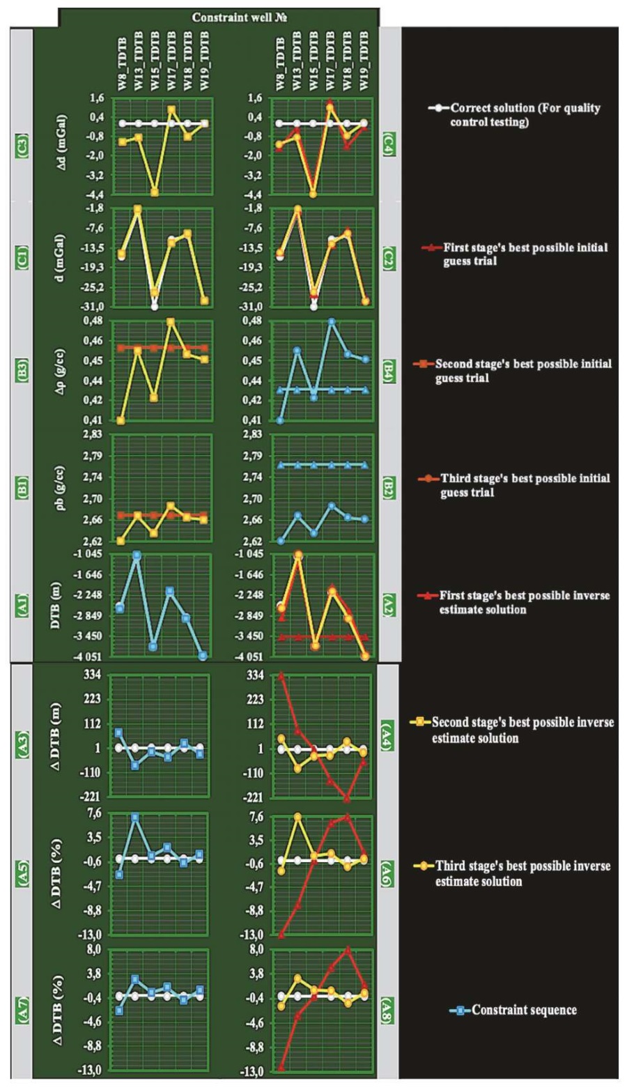
Fig. 10. The data analysis, which involves a three-stage inversion scheme
to identify three most appropriate solutions
when the correlation is made with the accessible-well quality control tests.
Red, blue and yellow sequences represent the first, second and third most appropriate solutions of a three-stage method. The desired quality solutions are shown as green circles. Table 2 displays the list of abbreviations.
Рис. 10. Анализ данных, включающий трехэтапную схему инверсии
для определения трех наиболее подходящих решений
при корреляции с проверкой контроля качества доступных скважин.
Красные, синие и желтые линии – соответственно первое, второе и третье наиболее подходящие решения трехэтапного метода. Зеленые кружки – необходимые качественные решения. В табл. 2 приведен список сокращений.
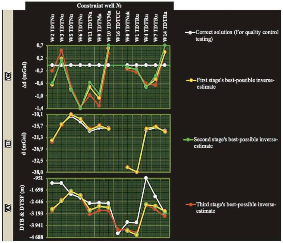
Fig. 11. Another test, which ensures the quality control
of the three-stage inverse most appropriate depth model solutions
using thirteen non-accessible basement-constrained wells.
With minimal data misfit, this test successfully produced optimal basement depths (as compared to the largest depths) for almost all of these wells in various sedimentary formations. The locations of these constrained wells are shown in the Bouguer anomaly map with orange circles. Table 2 displays a list of abbreviations.
Рис. 11. Результаты проверки контроля качества трехэтапной инверсионной модели
для наиболее оптимальных глубин на примере 13 скважин.
При минимальном искажении данных проверка позволяет получить показатели оптимальной глубины залегания фундамента (по сравнению с наибольшими глубинами) почти для всех скважин в различных осадочных пластах. Расположение этих скважин на карте аномалий Буге обозначено оранжевыми кружками. Табл. 2 содержит перечень сокращений.
Figs 10, 11, indicate that the most appropriate inversion trials on the three-stage inversion scheme provided inversely computed parameters for depth, depth misfit, density, density contrast, Bouguer anomaly, and Bouguer anomaly misfit throughout the six constrained wells, as illustrated in graphs A1–A8, B1–B4, and C1–C4, respectively. First, we performed a depth correlation quality control (A1 and A2) for the sixth optimal modeling trial on the three-stage inversion scheme and assessed the depth misfit (graphs A3–A8). These assessments show that the most appropriate constrained density assumption improves the optimal inverted depth model. Next, we examined the constrained well density and density contrast (graphs B1–B4) to determine how the lateral distribution of basement density influences depth gain with minimal error. Finally, we tested the Bouguer misfit as a result of anomalous correlation. These Bouguer tests with a virtually minimal misfit show that the depth-density model is optimal, and our scheme generates appropriate depth and density for the study area.
In-depth analysis of indirectly constrained wells. According to the well data analysis illustrated in the graphs (A2 and A4) in Fig. 10, the most appropriate sixth optimal inverse trial of the mean basement depth model (highlighted in graph B, Fig. 4) yielded the least error in the model calculations for the first stage of our inversion scheme for six constrained basement wells. The basement depth model of our schematic third stage was further optimized with an estimated depth sequence, reducing the misfit with the best correlation to actual depths (Fig. 10, graph A4). This depth misfit sequence reveals the best quality control and shows that our schematic third-stage inversion optimal nineteenth depth model trial (highlighted in graph B, Fig. 4) has minimum inaccuracy.
As shown in Fig. 10, graph A6, the most appropriate depth misfit trial for the first and third stages of our inversion scheme yielded a percentagely inversed depth misfit sequence estimated individually for each of the six wells based on their actual depths.
Graph A8 in Fig. 10 also displays percentage coefficients of variations for six constrained wells with optimal depth sequence estimates, recalculated using the actual mean basement depth. This re-estimation scenario is used for the first-stage sixth optimal depth misfit trial and the the third-stage nineteenth trial.
Within the six controlled wells, the third-stage optimal nineteenth constrained mean density trial, highlighted in graph C in Fig. 4, is distributed by lateral density sequence as depicted in Fig. 10, graphs B1 and B2.
Fig. 10, graph C4, illustrates the data misfit for six constrained wells, revealing the minimal misfit sequence that constrains the optimal basement depth. In addition, as depicted in Fig. 11 (graph C), this data misfit sequence yields nearly optimal estimates of basement depths which are larger than the actual depths to different sedimentary formations exposed in the cross-sections at the locations of the rest thirteen wells.
2D model extraction procedure for evaluation of optimality of 3D models. Figs 12, 13, 14, 15, 16 display the two-dimensional gravity inversion investigation at thirteen 2D seismic line positions in the study area. This investigation is based on the two-dimensional gravity models extracted from the optimal three-dimensional gravity model obtained for the study area by our schematic third-stage sixth inverse optimal modeling trial. This trial has minimal inverse modeling and data misfit errors. This data, with nearly zero mean misfits, reveals that the 2D extracted models have the most appropriate depth, density, and density contrast values.
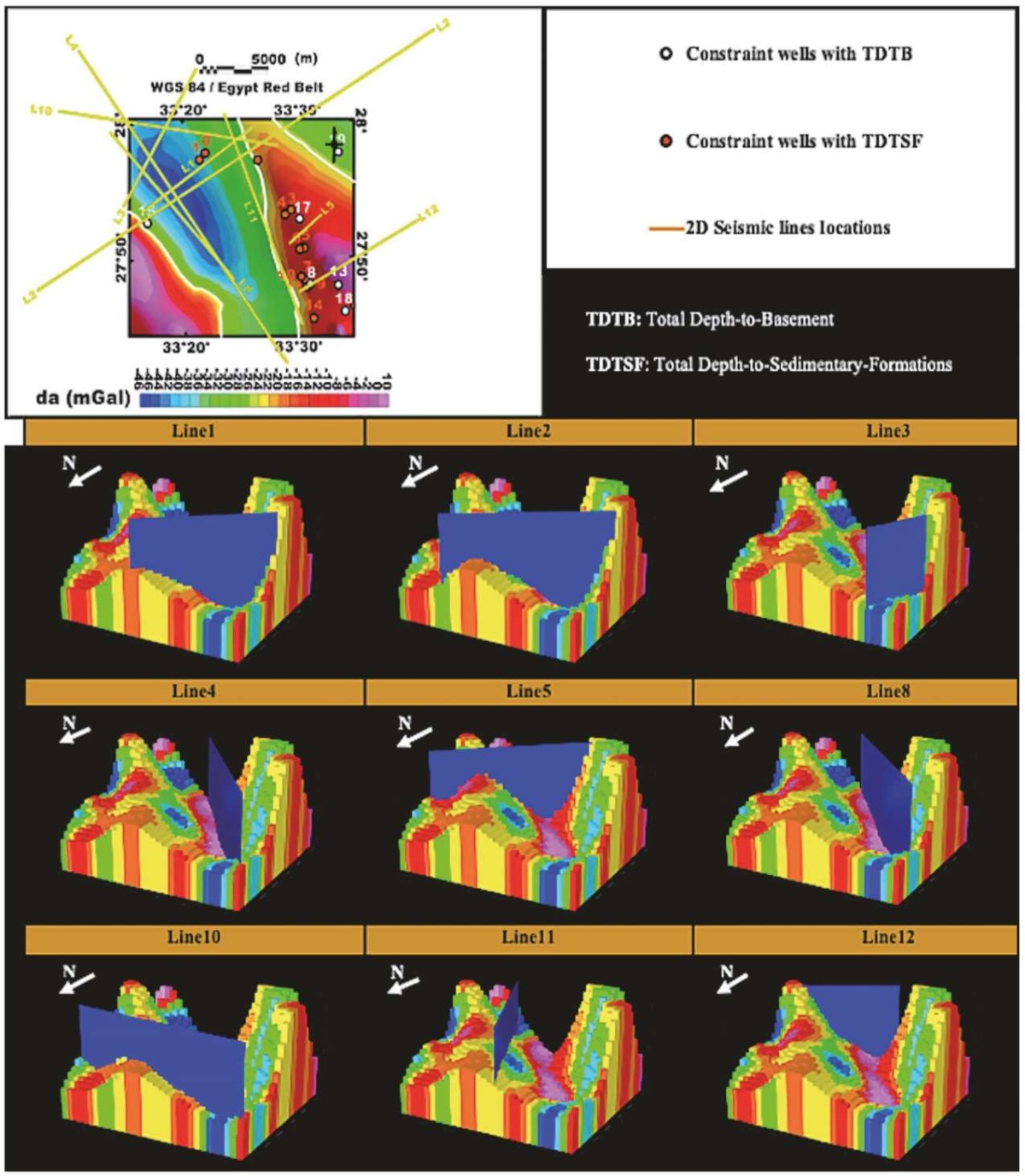
Fig. 12. 3D depth-density model at nine seismic lines.
Рис. 12. Глубинно-плотностная 3D-модель на девяти сейсмических профилях.
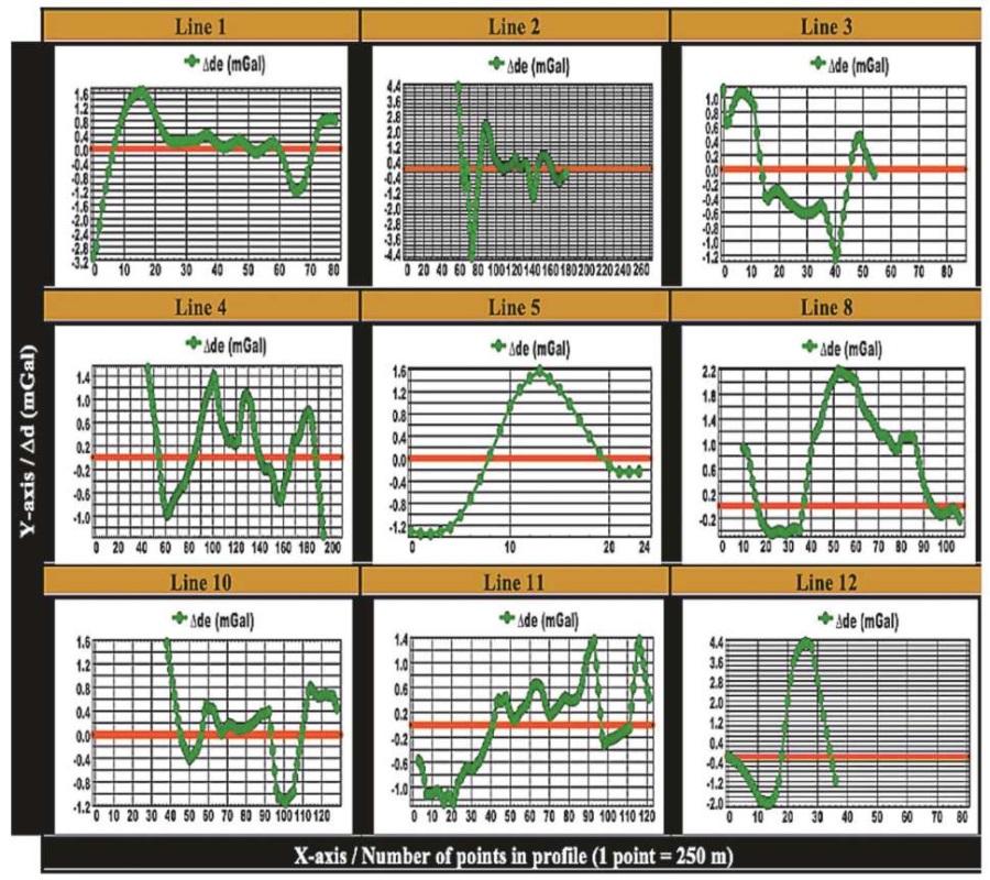
Fig. 13. Mismatch of Bouguer anomalies and seismic lines.
Рис. 13. Несовпадение аномалий Буге и сейсмических профилей.
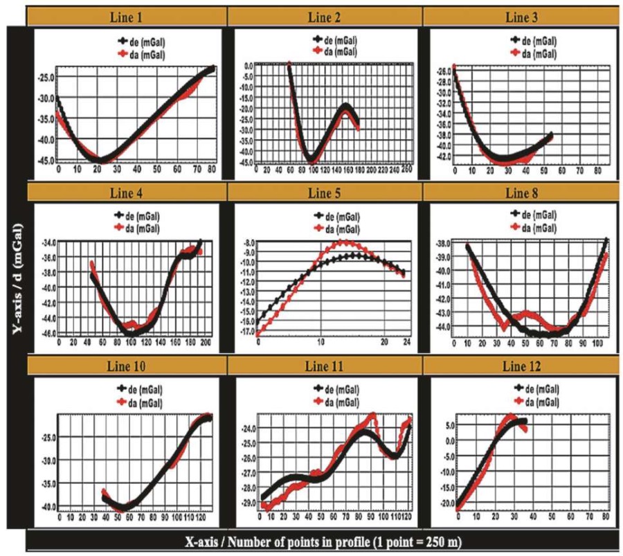
Fig. 14. Correlation between the calculated and observed Bouguer anomalies
at seismic line locations.
Рис. 14. Корреляция между расчетными и наблюдаемыми аномалиями Буге
в местах расположения сейсмических профилей.
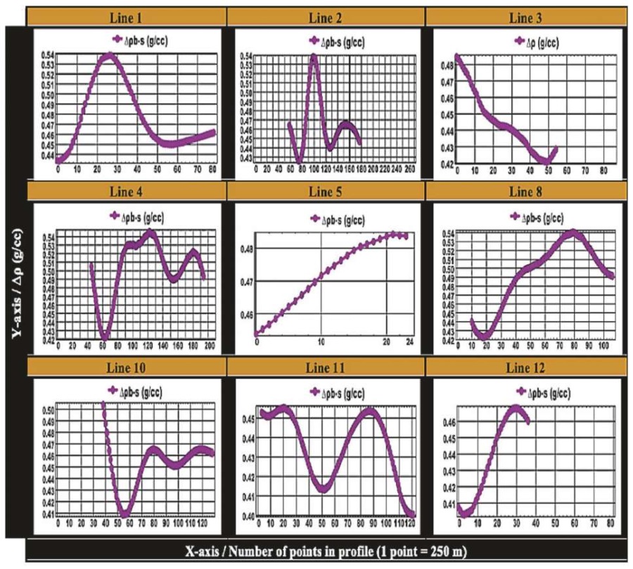
Fig. 15. Basement-sediment density-contrast interface at seismic line location.
Рис. 15. Изменение плотности на границе раздела фундамент – осадки
в местах расположения сейсмических профилей.
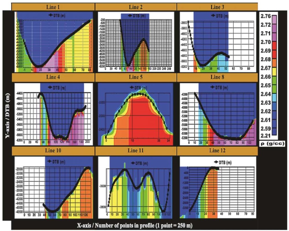
Fig. 16. 2D basement complex depth-density model at seismic line location.
In addition to the possibility of obtaining basement depth and lateral density distribution for various seismic line locations it is demonstrated the ability of the process to determine, with minimal data misfit, the optimal density contrast between basement and sediment.
Рис. 16. Комплексные глубинно-плотностные 2D-модели фундамента
в местах расположения сейсмических профилей.
В дополнение к возможности получения глубин фундамента и горизонтального распределения плотности для различных участков жирной линии (построенной по сейсмическим данным и разграничивающей фундамент и осадки) показана способность процесса определять с минимальными искажениями оптимальный скачок плотности между фундаментом и осадками.
Identification of tectonic features. The basement relief in this area, obscured with salt diapers in 2D seismic interpretation, was identified with the help of the recovered optimal 3D depth-density model at nine seismic lines obtained from inverse analysis of the Bougeur anomalies.
Geological insights for hydrocarbon studies were gained from analyzing the fully recovered optimal 3D residual Bouguer image of the deep sedimentary structure above the basement relief in the study area.
The fault planes on both sides of the study area may represent ideal paths for hydrocarbon migration. The sedimentary cover thickness in the central basinal area causes significant pressure, which may provide hydrocarbon migration along the fault planes on both sides of the study area with a high chance of hydrocarbon sealing in the fault traps thereon. This is due to the shallow basement complex in the study area and the impermeable sedimentary strata of the lithological column. As the basement blocks are exposed in the sedimentary section, they create many fault traps along the fault planes, which in turn produce small half-grabens and protracted sub-basins above the basement complex.
According to the lithostratigraphic column, the deep reservoir in El Zeit is made up of Nubia sandstone, which was formed by the tectonically active regional basement complex.
The best-estimated basement relief reveals that there are three main basement blocks in the study area: a downthrown block in the middle that created the basinal structure of the graben system, similar to the El Zeit basin which is 6453 m deep, and upthrown blocks on the western and eastern flanks with zero depths, similar in origin to the Gebel Zeit and Esh-Mellaha mountains.
A three-stage gravity inversion scheme was proposed to recover optimal solutions of the basement depth-density model for the southwestern part of the Gulf of Suez in the Gebel Zeit area. The challenge was to increase the validity of the scheme and improve the quality of the model to obtain the optimized depth-density model solutions that are best correlated to prior geologic information with the minimum error estimation. The scheme relied on a scenario without accessible wells as direct constraints in the direct modeling but with those in analyzing the inverse results as indirect quality controls. The inversion process constraint of DC shift force mean error is zero, and zero regional offset controlled the recovery of the inverse model with the minimal residual Bouguer gravity data misfit estimates.
Three most appropriate models were evaluated from the three stages, revealing an optimal scheme with gradually estimated error in depth-density model calculations following this root-mean-square deviation coefficient of variance sequence (6.4, 1.78, and 1.63 %). After analyzing and evaluating the entire study area, the optimality was shown for certain spots with thirteen drilled wells and nine seismic lines. This focused analysis showed the optimally recovered three-dimensional depth-density model, best correlated with geological prior information, represented by depth misfit estimated from the actual basement total depths of the six basement wells distributed within the range of 1.24–8.00 % relative to the actual mean basement depth of these wells.
After conducting depth inversion trials within three stages with three different scenarios, the subsurface model for basement depth was optimized with a minimal error of 1.63 %. The model yields an image for the mean basement depth of 3534.6 m, ranging from 0 to 6453.2 m, with an outcropping visible on the surface. Additionally, the basement complex lateral density model was inversely modeled resulting in the 1.63 % depth minimal error and imaging the prevalence of granitic basement rocks in the study area, with density ranging from 2.6706 to 2.7558 g/cc and a mean value of 2.6706 g/cc.
The 3D depth-density model helped to overcome the 2D seismic interpretation problem of delineating the basement relief in the area obscured with salt diapers. It also provided geological insight into the study area, revealing the presence of graben systems and the formation of half grabens.
Tectonically, this study aims to determine the most accurate model image of the graben system for the study area. The basement relief image shows the stratigraphic framework of a graben, which is bounded by two major faults that extend from the surface to the depth. This relief is on average roughly 3.481 meters deep. With a mean density contrast of 0.45 g/cc, the sedimentary section is somewhat less dense than the basement complex, which has a mean density of 2.71 g/cc. According to this model, the El Zeit’s deep basinal area has a maximum sedimentary cover thickness of 6453.2 meters, and its basement-sedimentary interface consists of two long, deep-to-shallow normal faults covered by a thick sedimentary cover. Sediment pressure increases throughout the basin. This enhances the probability of hydrocarbon migration through the fault planes and its capture in fault traps. Shallow-basement tectonic criteria and impermeable sedimentary strata in the lithologic column are favourable for hydrocarbon entrapment.
This scheme is proposed for implementation in a newly explored region with limited prior information; it has a high likelihood of recovering the approximately reliable and accurate solutions for the inverse model with a minimal error rate of 1.63 %. Future plans include conducting back-stripping to obtain a comprehensive three-dimensional density-depth model of the study area which enhances our understanding of the geological structure and aids in identifying potential hydrocarbon traps. Additionally, petroleum studies are planned to assess the presence of hydrocarbon reservoirs in the study area, highlighting the potential for hydrocarbon accumulation in specific locations.
Researcher Ahmed G.M. Hassan appreciates the financial support from the Arabic Republic of Egypt, represented by the Central Department of Missions under the Cultural Affairs and Missions Sector at the Ministry of Higher Education of Egypt, covering his living expenses along with his study at the Saint Petersburg State University in Russia. Also, he appreciates the chance given to him by the Russian Federation, represented by the Ministry of Higher Education, to be enrolled in a PhD Program by a scholarship without tutorial fees.
A.G.M. Hassan contributed significantly to planning and designing a study, conceptualization, methodology, software utilization, formal analysis, interpretation, resource organization, and original draft preparation.
K.S.I. Farag provided an equivalent contribution by critically reassessing the intellectual content of a specific field of study, visualization, validating the findings, and participating in the writing process through review and editing.
A.A.F. Aref and A.L. Piskarev acted as supervisors.
А.Г.М. Хассан внес значительный вклад в планирование и разработку исследования, концептуализацию, выбор методологии, работу с программным обеспечением, формальный анализ, интерпретацию полученных данных и подготовку первоначального проекта публикации.
Эквивалентный вклад принадлежит К.С.И. Фарагу, который критически оценил интеллектуальное содержание конкретной области исследования, визуализировал и подтвердил полученные результаты, а также принял участие в процессе написания работы посредством рецензирования и редактирования.
А.А.Ф. Ареф и А.Л. Пискарев выступили руководителями исследования.
Авторы заявляют об отсутствии конфликта интересов. Авторы прочли и одобрили финальную версию рукописи перед публикацией.
The authors declare that they have no conflicts of interest to declare. The authors read and approved the final manuscript.
1. Aboud E., Salem A., Ushijima K., 2005. Subsurface Structural Mapping of Gebel El-Zeit Area, Gulf of Suez, Egypt Using Aeromagnetic Data. Earth Planets Space 57, 755–760. https://doi.org/10.1186/BF03351854.
2. Abuzied S.M., Kaiser M.F., Shendi E.H., Abdel-Fattah M.I., 2020. Multi-Criteria Decision Support for Geothermal Resources Exploration Based on Remote Sensing, GIS and Geophysical Techniques along the Gulf of Suez Coastal Area, Egypt. Geothermics 88, 101893. https://doi.org/10.1016/j.geothermics.2020.101893.
3. Afifi A.S., Moustafa A.R., Helmy H.M., 2016. Fault Block Rotation and Footwall Erosion in the Southern Suez Rift: Implications for Hydrocarbon Exploration. Marine and Petroleum Geology 76, 377–396. https://doi.org/10.1016/j.marpetgeo.2016.05.029.
4. Almalki K.A., Mahmud S.A., 2018. Gulfs of Suez and Aqaba: New Insights from Recent Satellite-Marine Potential Field Data. Journal of African Earth Sciences 137, 116–132. https://doi.org/10.1016/j.jafrearsci.2017.10.004.
5. Bendaoud A., Hamimi Z., Hamoudi M., Djemai S., Zoheir B. (Eds), 2019. The Geology of the Arab World – An Overview. Springer, Cham, 546 p. https://doi.org/10.1007/978-3-319-96794-3.
6. Crossley D., Hinderer J., Riccardi U., 2013. The Measurement of Surface Gravity. Report on Progress in Physics 76, 046101. https://doi.org/10.1088/0034-4885/76/4/046101.
7. Dadak B., 2017. Inversion of Gravity Data for Depth-to-Basement Estimate Using the Volume and Surface Integral Methods: Model and Case Study. PhD Thesis (Master of Science in Geohysics). Salt Lake City, 84 p.
8. Elgammal R., Orabi O., 2019. Coniacian-late Campanian Planktonic Events in the Duwi Formation, Red Sea Region, Egypt. Journal of Geology & Geophysics 7, 456. https://doi.org/10.4172/2381-8719.1000456.
9. Fan D., Li S., Li X., Yang J., Wan X., 2021. Seafloor Topography Estimation from Gravity Anomaly and Vertical Gravity Gradient Using Nonlinear Iterative Least Square Method. Remote Sensing 13 (1), 64. https://doi.org/10.3390/rs13010064.
10. Faris M., Ghandour I.M., Zahran E., Mosa G., 2015. Calcareous Nannoplankton Changes during the Paleocene-Eocene Thermal Maximum in West Central Sinai, Egypt. Turkish Journal of Earth Sciences 24 (5) 475–493. https://doi.org/10.3906/yer-1412-34.
11. Feng X., Wang W., Yuan B., 2018. 3D Gravity Inversion of Basement Relief for a Rift Basin Based on Combined Multinorm and Normalized Vertical Derivative of the Total Horizontal Derivative Techniques. Geophysics 83 (5), G107–G118. https://doi.org/10.1190/geo2017-0678.1.
12. Florio G., 2018. Mapping the Depth to Basement by Iterative Rescaling of Gravity or Magnetic Data. Journal of Geophysical Research: Solid Earth 123 (10), 9101–9120. https://doi.org/10.1029/2018JB015667.
13. Florio G., 2020. The Estimation of Depth to Basement under Sedimentary Basins from Gravity Data: Review of Approaches and the ITRESC Method, with an Application to the Yucca Flat Basin (Nevada). Surveys in Geophysics 41, 935–961. https://doi.org/10.1007/s10712-020-09601-9.
14. Hadada Y.T., Hakimi M.H., Abdullah W.H., Kinawy M., El Mahdy O., Lashin A., 2021. Organic Geochemical Characteristics of Zeit Source Rock from Red Sea Basin and Their Contribution to Organic Matter Enrichment and Hydrocarbon Generation Potential. Journal of African Earth Sciences 177, 104151. https://doi.org/10.1016/j.jafrearsci.2021.104151.
15. Jessell M., Aillères L., Kemp De E., Lindsay M., Wellmann F., Hillier M., Laurent G., Carmichael T., Martin R., 2014. Next Generation Three-Dimensional Geologic Modeling and Inversion. In: K.D. Kelley, H.C. Golden (Eds), Building Exploration Capability for the 21st Century. Special Publications of the Society of Economic Geologists 18, p. 261–272. https://doi.org/10.5382/SP.18.13.
16. Li Y., Oldenburg D.W., 1998. 3-D inversion of Gravity Data. Geophysics 63 (1), 109–119. https://doi.org/10.1190/1.1444302.
17. Maag E., Li Y., 2018. Discrete-Valued Gravity Inversion Using the Guided Fuzzy. Geophysics 83 (4), G59–G77. https://doi.org/10.1190/geo2017-0594.1.
18. Makled W.A., Ashwah A.A.E.E., Lotfy M.M., Hegazey R.M., 2020. Anatomy of the Organic Carbon Related to the Miocene Syn-Rift Dysoxia of the Rudeis Formation Based on Foraminiferal Indicators and Palynofacies Analysis in the Gulf of Suez, Egypt. Marine and Petroleum Geology 111, 695–719. https://doi.org/10.1016/j.marpetgeo.2019.08.048.
19. Mallesh K., Chakravarthi V., Ramamma B., 2019. 3D Gravity Analysis in the Spatial Domain: Model Simulation by Multiple Polygonal Cross-Sections Coupled with Exponential Density Contrast. Pure and Applied Geophysics, 176, 2497–2511. https://doi.org/10.1007/s00024-019-02103-9.
20. Oldenburg D.W., 1974. The Inversion and Interpretation of Gravity Anomalies. Geophysics 39(4), 526–536. https://doi.org/10.1190/1.1440444.
21. Pham L.T., Oksum E., Do T.D., 2018. GCH_Gravinv: A MATLAB-Based Program for Inverting Gravity Anomalies over Sedimentary Basins. Computers & Geosciences 120, 40–47. https://doi.org/10.1016/j.cageo.2018.07.009.
22. Preston L., Poppeliers C., Schodt D.J., 2020. Seismic Characterization of the Nevada National Security Site Using Joint Body Wave, Surface Wave, and Gravity Inversion. Bulletin of the Seismological Society of America 110 (1), 110–126. https://doi.org/10.1785/0120190151.
23. Radwan A.E., Abdelghany W.K., Elkhawaga M.A., 2021. Present-Day In-Situ Stresses in Southern Gulf of Suez, Egypt: Insights for Stress Rotation in an Extensional Rift Basin. Journal of Structural Geology 147, 104334. https://doi.org/10.1016/j.jsg.2021.104334.
24. Ren Z., Chen C., Pan K., Kalscheuer T., Maurer H., Tang J., 2017. Gravity Anomalies of Arbitrary 3D Polyhedral Bodies with Horizontal and Vertical Mass Contrasts. Surveys in Geophysics 38, 479–502. https://doi.org/10.1007/s10712-016-9395-x.
25. Said R. (Ed.), 2017. The Geology of Egypt. Routledge, London, 734 p. https://doi.org/10.1201/9780203736678.
26. Silva J.B.C., Santos D.F., Gomes K.P., 2014. Fast Gravity Inversion of Basement Relief. Geophysics 79 (5), G79–G91. https://doi.org/10.1190/GEO2014-0024.1.
27. Stolk W., Kaban M., Beekman F., Tesauro M., Mooney W.D., Cloetingh S., 2013. High Resolution Regional Crustal Models from Irregularly Distributed Data: Application to Asia and Adjacent Areas. Tectonophysics 602, 55–68. https://doi.org/10.1016/j.tecto.2013.01.022.
28. Van Dijk J., Al Bloushi A., Ajayi A.T., De Vincenzi L., Ellen H., Guney H., Holloway Ph., Khdhaouria M., McLeod I.S., 2019. Hydrocarbon Exploration and Production Potential of the Gulf of Suez Basin in the Framework of the New Tectonostratigraphic Model. In: Proceedings of the SPE Gas & Oil Technology Showcase and Conference 2019 (October 21–23, 2019, Dubai, UAE). SPE, SPE-198622-MS. https://doi.org/10.2118/198622-MS.
29. Wu L., 2016. Efficient Modelling of Gravity Effects Due to Topographic Masses Using the Gauss-FFT Method. Geophysical Journal International 205 (1), 160–178. https://doi.org/10.1093/gji/ggw010.
30. Wu L., 2018. Efficient Modeling of Gravity Fields Caused by Sources with Arbitrary Geometry and Arbitrary Density Distribution. Surveys in Geophysics 39, 401–434. https://doi.org/10.1007/s10712-018-9461-7.
31. Wu L., 2019. Fourier-Domain Modeling of Gravity Effects Caused by Polyhedral Bodies. Journal of Geodesy 93, 635–653. https://doi.org/10.1007/s00190-018-1187-2.
32. Wu L., Lin Q., 2017. Improved Parker’s Method for Topographic Models Using Chebyshev Series and Low Rank Approximation. Geophysical Journal International 209 (2), 1296–1325. https://doi.org/10.1093/gji/ggx093.
33. Youssef M., El-Sorogy A., El-Sabrouty M., Al-Otaibi N., 2016. Invertebrate Shells as Pollution Bio-Indicators, Gebel El-Zeit Area, Gulf of Suez, Egypt. Indian Journal of Geo-Marine Sciences 45 (5), 687–695.
7/9 Universitetskaya Emb, Saint Petersburg 199034
530 El Maadi, Cairo 11728
Abbassia, Cairo 11566
530 El Maadi, Cairo 11728
7/9 Universitetskaya Emb, Saint Petersburg 199034
Hassan A., Farag K., Aref A., Piskarev A.L. METHODS FOR 3D INVERSION OF GRAVITY DATA IN INDENTIFYING TECTONIC FACTORS CONTROLLING HYDROCARBON ACCUMULATIONS IN THE EL ZEIT BASIN AREA, SOUTHWESTERN GULF OF SUEZ, EGYPT. Geodynamics & Tectonophysics. 2024;15(2):0751. https://doi.org/10.5800/GT-2024-15-2-0751. EDN: AAFHCI


Editor-in-Chief
Sklyarov E.V.664033, Irkutsk, Lermontova St., 128,
IEC SB RAS Institute of the Earth's crust
E-mail.: gt@crust.irk.ru
tel.: 8 3952 425422
Processing of personal data


